
Contributed by: Eugen Stripling, Bart Baesens, Seppe vanden Broucke
This article first appeared in Data Science Briefings, the DataMiningApps newsletter. Subscribe now for free if you want to be the first to receive our feature articles, or follow us @DataMiningApps. Do you also wish to contribute to Data Science Briefings? Shoot us an e-mail over at briefings@dataminingapps.com and let’s get in touch!
The comparison of two groups is one of the most frequently encountered situations in research [1], [2], [3], [4]. The goal is to investigate whether there is a significant difference between two groups of interest. Here, group is a synonym for population. In practice, researchers usually work with samples that are taken from the two populations. Even though researchers’ attempts to keep extraneous effects on the data to a minimum, random variability often still contaminates the data, and the resulting “noise” can disguise the true nature of the two groups [1]. Therefore, researchers rely on statistical methods that help them to investigate the true relationship between the two populations based on the samples. Many statistical methods exist to do so, but the t test is undoubtedly the most popular statistical hypothesis testing procedure for two-sample comparison. Note that the t test was developed under the frequentist paradigm, which interprets probabilities as being the limit of relative frequencies.
Bayesian estimation (BEST) as proposed by Kruschke [1] is an interesting alternative to the frequentist approach; it offers a coherent and flexible inference framework that provides richer information than null hypothesis significance testing (NHST). In contrast to NHST, Bayesian methods estimate a joint probability distribution of the parameters. This distribution offers a much richer foundation for inference, which in turn also allow a more straightforward interpretation of the statistical outcome [1]. A key characteristic of the BEST approach for two groups is that the data are by default modeled as a t distribution instead of a normal one, hence making the model more robust against outliers. That is because the t distribution possesses heavier tails, and therefore better accommodates outliers.
In Bayesian, probability is a measure for the degree of belief, indicating how credible a candidate possibility is [5]. The probability distribution is then the distribution of credibilities over all possibilities, reflecting our certainty in particular candidate possibilities. In the two-sample comparison context, we estimate the values of certain parameters that are related to the two groups. Thus, “candidate possibilities” refer to the space of possible parameter values. In Bayesian, the aim is to estimate the so-called posterior distribution, which is the probability distribution of the parameters taking into account the data. In order to estimate the posterior, users first have to specific their prior beliefs, or the prior credibility distribution, about possible parameter values before seeing the data. After the data have been collected, the prior beliefs are updated using the Bayes’ rule to obtain the posterior distribution. In other words, the posterior is the distribution of credible parameter values after seeing the data, and the Bayes’ rule reallocates our prior beliefs in a rigorous, mathematical manner based on the observed data [1].
An important distinction to the frequentist approach is that the Bayesian approach fixes the data and treats the parameters of interest as random variables, whereas the frequentist framework does the exact opposite [5]. Treating parameters as a random variable is preferable, because its probability distribution reflects our (un)certainty in possible parameter values. Since Bayesian methods work with distributions, more information is processed in the estimation procedure, and consequently allows a richer inference. Moreover, the data are considered to be fixed in Bayesian. This makes intuitively sense since these are the data we have actually observed, and the samples are viewed to be representative of the populations. There is no doubt about it. Taking more samples should bring us closer to the ground truth, and every sample that is taken is ultimately a representation of the ground truth. On the contrary, the frequentist paradigm assumes that the parameters are fixed and the data are random, which stem from the distribution with the fixed parameters. In the frequentist framework, inference is based on the assumption that the data are considered to be one realization out of an infinite number of possibilities. In practice, however, taking multiple samples is often impossible due to time and cost constraints. Thus, researchers are often limited to make inference based on one sample. And in NHST, the p value is a measure of how extreme the observed sample is (i.e. its resulting test statistic) under a certain null hypothesis. According to [1], [5], the concept of p values for decision making is fundamentally ill-defined, because it entirely depends on the (implicit) sampling intention of the researcher. In other words, sampling intention influences the p value, whereas Bayesian inference is not affected by this intention.
To apply Bayesian methods, one has to specify a descriptive model of the data, which possesses certain parameters to express the characteristics of the involved distributions. These parameters carry certain meanings, and estimating their posterior distribution allows researchers to answer their research questions [1]. In fact, the posterior is all that is needed to make statistical inference, since the posterior distribution of credible parameter values contains all necessary information [1], [5]. Before one can estimate the posterior, the user has to specific the prior distributions. Although at first it seems that specifying the priors forces extra effort on the users, but, in contrast to NHST, Bayesian methods make in this way the model assumptions about the data explicit [5]. Of course, reasonable priors must to be set that are accepted by the skeptical scientific audience [1]. Typically, non- or (mildly-)informative priors are set that are very wide and vague to assign all parameter values in the space (near) equal credibility. This way, the prior has little influence on the parameter estimation and even the modest amount of data will overwhelm the prior [1]. On the other hand, informative priors have to be justified to the skeptical scientific audience. Informative priors may be interesting to considered since they permit the incorporation of previous research findings into the analysis. When in doubt of the priors, Kruschke recommends to conduct a sensitivity analysis, i.e. investigating the influence on the posterior when using different priors in the model.
The BEST approach for the two-sample comparison models each group as a t distribution, where y1i and y2i are the observed data, denoted as D, of group 1 and 2, respectively. In the descriptive model (Figure 1), the parameters µ1, µ2 and σ1, σ2 respectively represent the means and standard deviations of the two groups. And the Greek letter (nu) ν ≥ 1 is the normality parameter that can be interpreted as a link to the normal distribution. That is, the larger ν, the more it converges to the normal shape, where a ν value near 30 is already a good approximation of the normal distribution. Large values of ν pull the probability mass towards the center, suggesting that the data appear to be normally distributed with no apparent outliers [1]. On the other hand, small values of ν shift more probability mass to the tails, enabling the t distribution to accommodate outliers. In Figure 1, the distributions with the blue superimposed histograms present the priors.
![Figure 1: General descriptive model of the BEST approach for two-sample comparison [1].](http://www.dataminingapps.com/wp-content/uploads/2016/03/figure1.jpg) |
Figure 1: General descriptive model of the BEST approach for two-sample comparison, source: [1].
The descriptive model can also be expressed mathematically [1]:
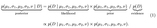 |
BEST’s default priors are defined very broad and vague so that the likelihood (i.e. the data contribution) has a strong influence on the parameter estimation. A detailed discussion and motivation for the choice of the default priors and their parameter settings are given in [1]. A difficulty arises with the term in the denominator, p(D), because for many models it cannot be computed analytically [1]. Therefore, a Markov chain Monte Carlo (MCMC) method is used in order to approximated the posterior without the need to compute the evidence, p(D). To carry out the computation, the R programming language [6] and the MCMC sampling language called JAGS (Just Another Gibbs Sampler) [7] are required. The MCMC sample, often referred to as the MCMC chain, is a sample of representative parameter values from the posterior. It is important to note that BEST simultaneously estimates the joint posterior distribution over the credible combinations of (µ1,σ1,µ2,σ2,ν) [1]. Based on the MCMC chain, various types of statistics can be computed to test multiple hypotheses of interest without having to correct for multiple testing [1], [5]! These statistics can be estimated with arbitrarily high precision. That is, the Law of Large Numbers shows its effects: the larger the MCMC chain, the higher the precision. Note however that BEST’s default settings for the MCMC should suffice for most cases.
To illustrate the BEST method, let’s consider one of Kruschke’s examples in which two groups of people take an IQ test. Group 1 (N1 = 47) gets administered a “smart drug”, whereas group 2 (N2 = 42) receives a placebo. The research question is: “Do people who take the smart drug perform better on the IQ test than those in the control group?” Although it is a fictitious example in which data were generated using two t distributions, it still resembles a realistic setting that could occur in practice. The histogram of the data can be seen in the upper right part of Figure 2, which clearly shows the presence of outliers. Executing the BEST analysis yields the MCMC chain, which contains representative parameter values sampled from the posterior. Plotting these parameter values as a histogram (left column of Figure 2) and computing simple statistics based on the MCMC sample (e.g. mean and mode) offers great insights into the distribution of credible parameter values, given the data.
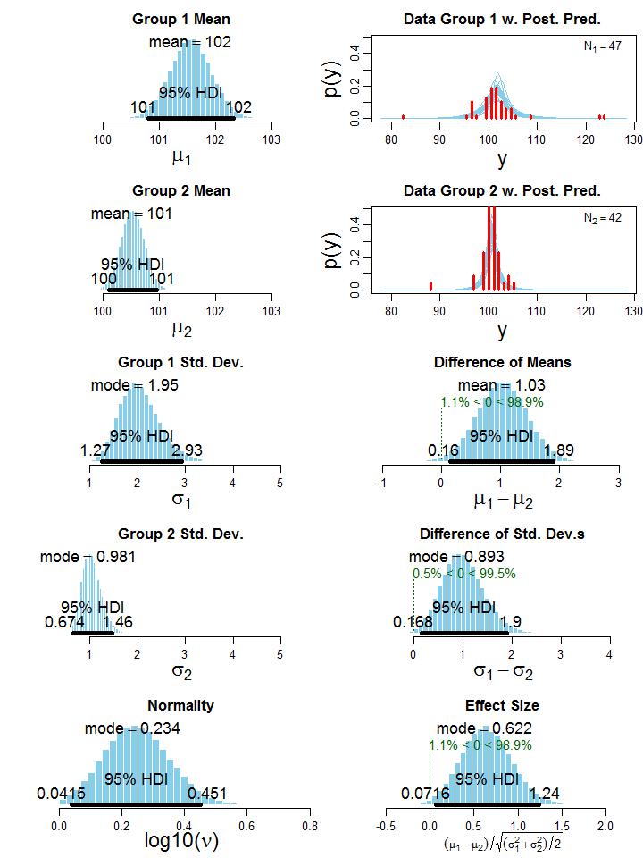 |
Figure 2: Histogram of the credible parameter values from the posterior. The 95% HDI (Highest Density Interval) indicates the interval of the most credible values, source: [1].
Note that the normality parameter ν is presented on the logarithmic scale (i.e. log10), because the shape of the t distribution changes considerably for small ν values but relatively little when ν is larger than 30 [1]. Thus, a log10(ν) = 0.234 corresponds to v ≈ 2, indicating that the t distributions of the two groups exhibit heavy tails to account for the outliers. In other words, it suggests that the data in the two groups are not normally distributed. The HDI on the histograms in Figure 2 denotes the highest density interval, revealing what range of parameter values are the most credible, given the data [1], [5]. For example, parameter values inside the 95% HDI have a higher probability density than any value outside the HDI, and total probability mass inside the HDI equals 95%. Recall Bayesian treats parameters as a random variable, and when using a 100(1 − α)% HDI it permits the follow interpretation: with a probability of 100(1 − α)%, the true value of the parameter lies between the two HDI limits. Such statement cannot be made with a NHST confidence interval. Now that we have a sample of credible values for the parameters µj and σj, j ∈ {1,2}, we can just take the difference between these parameters in each step of the MCMC chain to get the posterior distribution of credible values of the differences between means and standard deviations (third and fourth row of the right column in Figure 2). Since zero is not in the 95% HDI in both cases, we conclude that group 1 has a credibly larger mean (average difference of µ1 − µ2 = 1.03) and standard deviation (average difference of σ1 − σ2 = 0.893). This means, the smart drug credibly increases the IQ score on average. However, group 1 also has a credible larger standard deviation than group 2, meaning that some people may be positively and others may be negatively affected by the smart drug [1]. Kruschke also provides an estimate for the effect size (bottom right plot of Figure 2), but without including datarelated quantities such as sample sizes (i.e. N1 and N2; motivated in [1]). Nevertheless, we reach a similar conclusion as for the difference between means.
When applying a NHST t test to the same data, we obtain a test statistic value of t = 1.62 with a two-sided p value of 0.110 (in fact, this is the Welch two-sample t test to accommodate unequal variances). Hence, the conclusion is not to reject the null hypothesis at a significant level of α = 5%. This implies that the means of the two groups are not significantly different, which contradicts the Bayesian analysis. Normally, one tests for equal variances beforehand in order to decide whether to use a t test that accounts for unequal variances. The NHST F test of the ratio of variances yields a F(46,41) = 5.72 with a p value < .001, hence reject the null hypothesis of equal variances. Unfortunately, carrying out two hypothesis tests inescapably requires to correct the significance level for multiple testing, imposing a much stricter criterion for rejecting the null hypothesis [1]. In our example, a Bonferroni correction would require to set the significance level of each test to α = 2.5%. Regarding the t test’s insignificance, the critical reader might say: “The t test is only designed for normal data, which clearly are not in this example.” Therefore, Kruschke carried out a resampling technique, which is the standard approach in NHST if the distributional assumption is violated. He concluded that the p value of the resampling test of the difference between means is 0.116 (close to the conventional test), and the p value for the difference between standard deviations is 0.072 (much larger than the conventional test, and not significant anymore). Despite using the resampling method to account for non-normality, NHST does not reject the null hypotheses (plural!), while Bayesian estimation clearly shows that there is a credible difference of means and standard deviations between the two groups.
Readers may now question which statistical inference is the correct one, but this is not the right question. According to Kruschke [1], the more important question is: “Which method provides the richest, most informative and meaningful results for any set of data?” and he also provides an immediate answer: “It is always Bayesian estimation.” This makes intuitively sense, because, unlike NHST, Bayesian methods estimate a whole distribution for the parameters of interest, hence more information is processed in the estimation allowing us to make a richer inference in the end.
The more important question is:
“Which method provides the richest,
most informative and meaningful results for any set of data?”
Here, we only scratched the surface of a vast research field. Due to the ease of interpretation and model flexibility, Bayesian methods are appreciated in many disciplines such as mathematics, physics, machine learning, medicine, engineering, law, and so on. Furthermore, in his article, Kruschke outlines how to precisely estimate the statistical power for various research goals retrospectively and prospectively. He further points out that the descriptive model in Figure 1 can easily be extended to multiple groups (i.e. Bayesian ANOVA), or to hierarchical models in which information is shared across group estimates (cfr. shrinkage effect).
More information on Bayesian estimation as proposed by Kruschke can be found on: http://www.indiana.edu/∼kruschke/BEST/. If you are now excited to carry out a robust Bayesian estimation on your data, there is an R package available, named BEST, that allows you to perform the analysis [8]. All in all, we conclude that Bayesian estimation provides a coherent and flexible inference framework that offers richer information, and it is an interesting alternative to the NHST t test.