
Contributed by: Eugen Stripling, Seppe vanden Broucke, Bart Baesens
This article first appeared in Data Science Briefings, the DataMiningApps newsletter. Subscribe now for free if you want to be the first to receive our feature articles, or follow us @DataMiningApps. Do you also wish to contribute to Data Science Briefings? Shoot us an e-mail over at briefings@dataminingapps.com and let’s get in touch!
In a previous post, we discussed Bayesian methods as an alternative to the classical t test for the comparison of two independent groups. In this post, we describe how so-called randomization tests can be applied to make the statistical analysis. Like the classical t test, this concept also belongs to the frequentist framework in which inference is based on p values. However, unlike the t test, randomization tests do not make any assumptions about the distribution of the data, and hence are regarded as a nonparametric technique [1]. Before we continue, it is important to note that the null hypothesis testing procedure discussed here assumes that the data stem from an experiment. For nonexperimental data, a similar method exists known as permutation tests, although they do not permit to draw such strong conclusions as with randomization tests.
Our aim is to test whether the two groups of interest are significantly different from each other. Under the null hypothesis, it is assumed that the two population means are equal, i.e., H0: µA = µB. Based on the collected samples, a test statistic is computed, and with the aid of its sampling distribution the p value is determined. If the p value is smaller than a predefined significance level (denoted as α and commonly set to 5%), the H0 is rejected and we conclude the alternative hypothesis (i.e., Ha: µA 6= µB); otherwise, there is not enough evidence to reject the H0. For the classical t test, the sampling distribution is the Student’s t distribution. Clearly, the p value is essential for decision making, but what exactly is the p value? A common misconception is that the p value indicates the likelihood of the H0 being true. The correct interpretation, however, is: given H0 is true, the p value is the probability that a test statistic value occurs that is at least as extreme as the observed one computed from the data at hand.
Besides being nonparametric, another strong suit of randomization tests is that they also do not require that the data are randomly sampled [1]. This is a convenient property in practice, because research has shown that the random sampling assumption is frequently violated in many domains (see, e.g., [2, 3, 4]). That is, a genuine random sample cannot be taken due to time or cost constraints, or is just infeasible. In such circumstances, statistical inference is made based on the subjects or experimental units that are available at that time. Despite not having a random sample, it nevertheless remains important for randomization tests that the data come from an experiment in which experimental units have been randomly assigned to treatments. Unlike random sampling, random assignment is usually under the control of the experimenter, which makes the fulfillment of the requirement much easier in practice.
With randomization tests, inference is made based on data permutations. To conduct a randomization test, first specify the test statistic of interest, e.g., the difference between arithmetic means. Second, permute the data and compute the test statistic for each data permutation, which in turn creates the so-called reference distribution [1]. Third, compute the p value based on the reference distribution and determine the significance using the decision logic outlined above.
Before providing an illustrative example of this inference framework, we need to stress the assumptions that are made in the H0 of a randomization test. The hypotheses in a randomization test are as follows [1, 2]:
- H0: The response of every experimental unit is the same regardless of which treatment the experimental unit has received.
For a two-sided test, the alternative hypothesis is
- Ha: The response of at least one experimental unit would have been different if the experimental unit had received another treatment.
To put it differently, under the H0, randomization tests assume exchangeability of experimental units. Thus, if the H0 was true, it would not matter to which treatment the experimental unit was assigned. We would observe the same response. In order to verify this, we rely on data permutations. Note that the hypotheses operate at the individual level, unlike the t test which only includes summary statistics of the samples. The p value—as a measure of evidence—then helps to assess how extreme the observed data permutation is. In other words, if H0 is true, the p value indicates the likelihood of the occurrence of the observed data permutation including those permutations that produce a more extreme test statistic value.
Now, suppose that we have two treatment groups, A and B, and four experimental units (designated as a, b, c, and d), which are randomly assigned to the two treatment groups.1 We conduct the experiment and measure the response of the experimental units. Assume we observed the following data [2]:
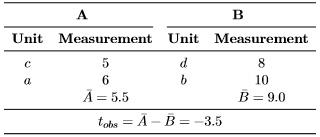 |
Our test statistic of interest is the difference between arithmetic means, where tobs is the observed test statistic value. Given the data, we can now generate all other data permutations and compute the corresponding test statistic value. Yet, how many data permutations do we need to generate? Let nA and nB be the sample sizes of the treatment group A and B, respectively. The number of all data permutations is then computed by P = N!/(nA!nB!), where N = nA + nB is the total sample size and the exclamation mark (!) denotes the mathematical operation known as factorial (e.g., 3! = 1 · 2 · 3 = 6). Thus, for our example, we have P = 4!/(2!2!) = 6 possible data permutations in total, which are as follows [2]:
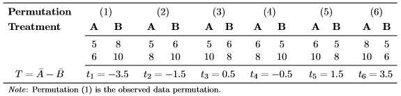 |
In other words, the test statistic, denoted as T, can possibly take six different values. The set of test statistic values is called the reference set [1] and represents the support of T: {ti} with i=1 to P. Computing the frequency of each value yields the reference distribution, which technically is the frequency distribution of T. Then, with the aid of the two-sided p value, it can be determined how extreme the observed data permutation is [1, 2]:
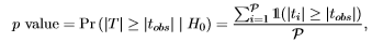 |
where the double barred 1(·) is the indicator function, i.e., it returns 1 if the input expression is true, 0 otherwise. Now, to compute the two-sided p value, simply determine the frequency of how many values (in absolute sense) in the reference set are equal to or larger than the observed test statistic value (i.e., |tobs| = 3.5) and divide it by the number of data permutations. In this example, the exact two-sided p value equals 2/6 or 33%. Hence, we conclude to not reject the H0 at a significance level of α = 5%. Note however that it is impossible to get a significant result at the 5% level with such small sample sizes, because the smallest, attainable p value is 1/P = 1/6 ≈ 16.7%. Yet, detecting that the observed data permutation produces an extreme test statistic value gives us an indication that there might be a difference between the two groups, but how can we prove it statistically? The most straightforward way to do so is to increase the sample size, but how many experimental units are needed in order to enable the randomization test to attain a twosided p value below 5%? For a balanced study such as in this example (i.e., nA = nB), it turns out that at least N = 8 experimental units are required. In this case, the smallest, attainable two-sided p value equals 2/70 = 2.86%. Any N value below 8 will have a two-sided p value larger than 5%.
In the above example, we were able to compute the exact p value, since all possible data permutations have been used to construct the reference set. This is referred to as the systematic approach [1]. The classical t test aims to approximate this exact p value. However, if the sample size is small, the t test approximates the exact p value poorly (i.e., p value ≈ 9%). That is mainly because that with such a small sample size (i.e., N = 4) the underlying assumptions of the t test are difficult to fulfill.
Randomization tests do not make any distributional assumptions about the data, but the resulting reference distribution will have a specific shape, which has a direct influence on the calculation of the p value. In fact, Ludbrook [4] demonstrated that the reference distribution can considerably deviate from the bell-shaped one. In his article, he showed that the reference distribution takes a skewed-bimodal shape. It is therefore important to keep in mind that the choice of a sensible test statistic is crucial [2].
To determine all data permutations is oftentimes very tedious or even infeasible, since the number of data permutations increases exponentially with the sample size. Therefore, Ludbrook [4] suggested to randomly sample from the reference distribution. A way to do so is to generate random data permutations in which the observed responses are randomly reassigned (without replacement) to one of the two groups. The test statistic is then computed based on the randomly generated data permutation. This is repeated K times in order to construct the reference distribution. Obviously, with random data permutations, it is only an approximation of the exact p value, but if N is large, this approach allows getting results in reasonable time, since typically KP. However, an important question is whether the p value based on random data permutations is also valid? In order to ensure validity, Edgington and Onghena [1] proposed the Monto Carlo randomization test in which tobs must be an element of the reference set so that only K−1 random data permutations are required to be generated.
An important note is also that randomization tests are conditional tests, meaning that inference is conditional on the given sample. For this reason, no generalization to the larger population is possible, unless a genuine random sample have been taken from the population. However, this is not a specific drawback of randomization tests, this applies to any statistical test. As previously mentioned, the random sampling assumption frequently cannot be fulfilled in practice. Edgington and Onghena [1] acknowledged this by explicitly addressing that the lack of random sampling is not a theoretical obstacle for the application of randomization tests. Without a random sample, they argued that inference is limited to the experimental units involved, and that inferences about treatment effects for other units must be made nonstatistically (not based on probabilities). This is often done in practice if no genuine random sample is acquirable.
Besides being nonparametric, easy to grasp and to implement (a Python 3 implementation is made available at: https://github.com/estripling/randomization tests), another more important advantage of randomization tests is that they allow users to easily specify any test statistic of interest and still remain a valid statistical test [2]. For example, in the presence of outliers, the difference between trimmed means can be used as test statistic, which is a robust alternative compared to arithmetic means.
In the previous post, we considered an example provided by Kruschke in which the research question was: “Do people who take the smart drug perform better on the IQ test than those in the control group?” Data were available from nA = 47 people who received the supposedly IQ-enhancement drug, and nB = 42 people received an placebo. Recall that there were outliers in the data. To test whether this is a significant difference between the two independent groups, a Monte Carlo randomization test has to be applied to approximate the exact two-sided p value, simply because the systematic reference set consists of P ‘ 4.5·1025 data permutations, which even with modern computers is too computationally expensive. When carrying out a Monte Carlo randomization test with K = 10,000 in which the test statistic is the difference between arithmetic means, a p value of 12.52% is obtained. Hence, we do not reject H0 at the α = 5% level. Note that we reached the same conclusion with the t test in the previous analysis. However, this test is naive, because of the presence of outliers in the data, which easily induce a distortion of the arithmetic means. In order to cope with the extreme observations, the difference between trimmed means (20% on each side) is a more appropriate test statistic. This test yields a p value of 1%, which leads to the rejection of the null hypothesis. Thus, the response of at least one person would have been different if (s)he had received the other treatment. This finding is in line with the previously conducted Bayesian analysis, which also accounted for outliers.
In conclusion, randomization tests provide an interesting alternative to the classical t test. They are straightforward and easy to understand—even if you do not have a strong background in statistics. Yet, their greatest advantage is that they easily allow users to make statistical inference with any test statistic of interest in a straightforward manner. Compared to the classical t test, this immense flexibility of randomization tests to easily adapt to given circumstances (e.g., presence of outliers) provides a tremendous enrichment of the null hypothesis significance testing framework.
References
- [1] E. Edgington and P. Onghena, Randomization Tests, 4th ed. Boca Raton, FL: Chapman & Hall/CRC, Taylor & Francis Group, 2007.
- [2] E. Stripling, “Distribution-free statistical inference for the comparison of central tendencies,” MSc thesis, Dept. LStat, KU Leuven, Leuven, Belgium, 2013.
- [3] R. B. May and M. A. Hunter, “Some advantages of permutation tests,” Canadian Psychology, vol. 34, no. 4, pp. 401–407, 1993.
- [4] J. Ludbrook, “Special article: Advantages of permutation (randomization) tests in clinical and experimental pharmacology and physiology,” Clinical and Experimental Pharmacology and Physiology, vol. 21, pp. 673–686, 1994.