
Contributed by: Sandra Mitrović
This article first appeared in Data Science Briefings, the DataMiningApps newsletter. Subscribe now for free if you want to be the first to receive our feature articles, or follow us @DataMiningApps. Do you also wish to contribute to Data Science Briefings? Shoot us an e-mail over at briefings@dataminingapps.com and let’s get in touch!
The performance of supervised predictive models is characterized by the generalization error, that is, the error, obtained on datasets different from the one used to train the model. More precisely, generalization error equals to expectation of predictive error over all datasets D and ground truth y and can be represented as: E D,y [L(y,f(x))], where f(x) is predicted outcome for an input x and L is the chosen loss function. Obviously, the goal is to minimize generalization error, which, for several most typical choices of loss function, can be decomposed as:
aL * Variance(x) + Bias(x) + bL * Noise(x)
Where factors aL and bL depend on the choice of a loss function L [1]. Bias measures systematic error, which stems from the predictive method used. Variance, on the other hand, is not related to the chosen modeling method, but rather to the dataset used. It represents fluctuations around the most commonly (in case of classification)/average (in case of regression) predicted value in different test datasets. Ideally, both bias and variance should be low, since high bias leads to under-fitting, which is inability of the model to fit the data (low predictive performance on train data), while high variance leads to over-fitting meaning that the obtained model is too much adjusted to the train data that it fails to generalize on test data (also known as “memorization” (of train data)). This, however, is not possible and hence, in practice, we have to make a trade-off between variance and bias.
Different types of models have different bias/variance profiles, e.g. Naïve Bayes classifier has low variance and high bias, while decision tree has low bias and high variance. Logistic Regression (LR) is a well-established method, which despite being fairly simple has been proven to have good performances [2]. On one side, this is beneficial since it facilitates interpretation of the model and obtained results. On the other side, having low variance (and high bias), makes it a limited method in terms of its expressive power. We can overcome this drawback by introducing more complex features, obtained as a Cartesian product of the original features. Logistic regression of order n (denoted as LRn) is defined as the logistic regression modeling the interactions of the n-th order (as defined in [3], although it can be, as well, defined to consider lower level interactions i.e. interactions of order ≤ n).
LRn allows modeling of much larger number of distributions, as compared to LR. Obviously, on smaller datasets this leads to over-fitting and different types of regularization are known in literature to penalize for the model complexity. But what happens in the case of really large datasets? It has been demonstrated that with the increase of training dataset, variance decreases and bias increases [4]. Hence, high variance of LRn would not be a problem, as long as bias could be controlled. Bias/variance profile of higher-order LR has been extensively investigated in [3], where LRn (for n=1,2,3) have been compared on 75 datasets from UCI repository. As it can be seen in the Figure 1 (borrowed from [3]), with increasing amount of data, higher-order LR perform better than the lower-order LR. In other words, with large enough datasets, as the order n increases, the bias of LRn descreases, This clearly motivates the usage of higher-order LR with large datasets.
Once again, it is very important to emphasize the amount of data observed (i.e. the number of instances). For example, based on the zoomed part of graph, if we would make a strict cutoff at any number of instances i, where i < 1000, due to the fact that LR1 learning curve has steeper decrease than both LR2 and LR3, we would conclude that LR1 performs the best (out of these three). As it can be seen from upper part of the figure, the same conclusion could be derived to the detriment of LR3 after sufficiently enough number of instances. However, for extensively large dataset, it is obvious that LR3 outperforms the other two. This phenomenon is due to the fact that lower-order logistic regressions have higher learning rate in the beginning of learning process.
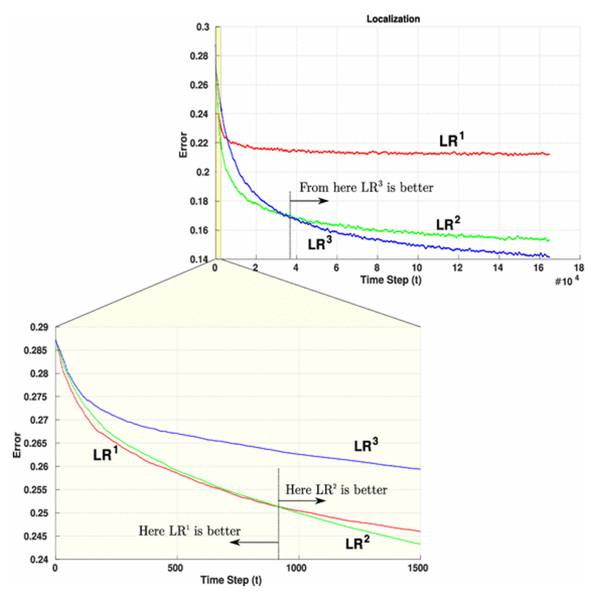
Figure 1: Learning curves of logistic regressions of different order plotted for increasing amount of data (an illustration from [3]). Click to view full size version.
References
- [1] Domingos, P. (2000). A unified bias-variance decomposition. In Proceedings of 17th International Conference on Machine Learning (pp. 231-238).
- [2] Baesens, B., Van Gestel, T., Viaene, S., Stepanova, M., Suykens, J., & Vanthienen, J. (2003). Benchmarking state-of-the-art classification algorithms for credit scoring. Journal of the operational research society, 54(6), 627-635.
- [3] Zaidi, N. A., Webb, G. I., Carman, M. J., & Petitjean, F. (2016). ALR n: Accelerated HigherOrder Logistic Regression. In Proceedings of European Conference on Machine Learning.
- [4] Brain, D., & Webb, G. I. (2002, August). The need for low bias algorithms in classification learning from large data sets. In European Conference on Principles of Data Mining and Knowledge Discovery (pp. 62-73). Springer Berlin Heidelberg.