
Contributed by: Eugen Stripling, Seppe vanden Broucke, Bart Baesens
This article first appeared in Data Science Briefings, the DataMiningApps newsletter. Subscribe now for free if you want to be the first to receive our feature articles, or follow us @DataMiningApps. Do you also wish to contribute to Data Science Briefings? Shoot us an e-mail over at briefings@dataminingapps.com and let’s get in touch!
The knapsack problem is popular in the research field of constrained and combinatorial optimization with the aim of selecting items into the knapsack to attain maximum profit while simultaneously not exceeding the knapsack’s capacity. We explain how a simple genetic algorithm (SGA) can be utilized to solve the knapsack problem and outline the similarities to the feature selection problem that frequently occurs in the context of the construction of an analytical model.
Genetic algorithms (GAs) are stochastic search algorithms that mimic the biological process of evolution enabling thereby users to solve complex optimization problems [1, 2]. They operate based on a population of chromosomes, where a chromosome represents a candidate solution. Genetic operators allow the population to evolve over time and to converge to the optimal solution. In the spirit of “survival of the fittest,” GAs are naturally designed to solve maximization problems in which chromosomes with high fitness are more likely to survive and the objective function is termed fitness function. The fitness function is a mathematical expression that evaluates the “quality” of a chromosome and steers the evolutionary search toward high fitness regions in the given search space. Note that the search space is usually a multi-dimensional space that consists of all candidate solutions. Two appealing properties of GAs are that they require no derivatives of the objective function and they are capable of performing global optimization. The former is in particular useful in situations in which, for example, no derivatives of the objective function exist and hence conventional techniques like gradient decent methods can–because of their very nature–not be applied. Given an unlimited amount of search time, GAs are able to find the global optimum in the search space. That is because they are less likely to get trapped in a local maximum due to their intrinsic stochastic mechanisms.
A SGA is probably the best known GA design, where chromosomes are represented as a binary string like ‘1010001’. The zeros and ones are the genes of a binary chromosome, and their meaning depends on the problem one tries to solve. To apply a SGA to a given optimization problem, an initial population of binary strings is first created in a random manner, subsequently the quality of each chromosome is evaluated using the fitness function. Based on the fitness values, a selection is done in such a way that high fitness chromosomes have a higher probability of being selected into the mating pool than low fitness chromosomes. The mating pool represents the foundation for breeding new candidate solutions. Chromosomes selected into the mating pools are also called parents [2].
Once the mating pool is created, a crossover is performed in order to exchange gene material between parents, which in turn creates new chromosomes, also called offspring or children. In SGAs, single-point crossover is a popular genetic operator that often used to perform the crossover for binary-encoded chromosomes (Figure 1). That is, with a probability pc, two parents are randomly selected from the mating pool, as well as a single crossover point between 1 and l−1 is randomly determined, where l is the length of the chromosome [2]. The children are then created by exchanging the genes of the parents after the crossover point.
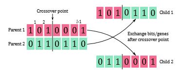
Figure 1: Single-point crossover, adapted from [2].
Next, mutation is applied to introduce a higher diversity into the population. The induced randomness of this genetic operator is useful because it helps to explore the search space and enables the SGA to escape local optima. A common operator is the bit-flip mutation (Figure 2). Similar to crossover, a chromosome is randomly selected with probability pm from the processed mating pool. The selected chromosome can either be a parent or a child. Then, a gene j of the selected chromosome is randomly picked and its value is flipped over, i.e., 0 becomes 1 and 1 becomes 0 [2]. A mutant is then a genetically modified chromosome as a result of the mutation operator. Thus, the mating pool now consists of parents (chromosomes that have been selected but neither undergo crossover nor mutation), children (new chromosomes resulting from crossing parents), and mutants (new chromosomes resulting from mutating parents or children). In the SGA implementation that we are going to use, pc and pm are by default set to 0.8 and 0.1, respectively. Thus, the lion’s share of the processed mating pool are likely children. In the next step, the fitness of children and mutants is evaluated.
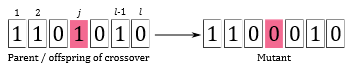
Figure 2: Bit-flip mutation [2].
After having applied the genetic operators, the population is updated to the next generation, and the SGAs converges to the (global) maximum one generation at a time. The update is conducted as follows: the mating pool obtained in the previous step is in principle the next generation. However, often SGAs utilize a mechanism called elitism which ensures that a certain proportion of the fittest chromosomes of the current population survives to the next generation. In other words, chromosomes with the lowest fitness in the mating pool are substituted with the fittest chromosomes of the current population. Once having done this, the mating pool becomes the next population, and the algorithm iterates. The advantage of elitism is that it increases the selective pressure among the chromosomes that compete for survival across generations and helps to maintain a high quality fitness level in the population, as well as keeping track of the best solution obtained so far. The steps outlined above are carried out repeatedly until a predefined number of maximum generations is reached or—commonly also applied—the best fitness function value has not improved for a predetermined number of generations. If a termination criterion is met, the SGA returns the fittest population member, which represents the final solution.
Given its zero-one encoding scheme, SGAs are naturally applicable to solve the knapsack problem. The knapsack problem aims to maximize the total profit for a selection of items, each with a profit pi and a weight wi, from a given item set of size n, while simultaneously preventing the violation of the constraint that the total weight of selected items exceeds the knapsack’s capacity W.
Let f(·) represent the fitness function and x = (x1,…,xn) be a binary vector, indicating selected items, i.e., xi = 1 if the ith item is selected into the knapsack, and xi = 0 otherwise (note that this example, as well as the following mathematical formulations and code, have been adapted from [2, 3]). The knapsack problem can be formally described as follows [2]:
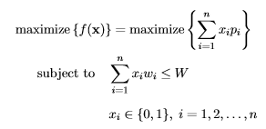
where we seek to find x∗ = argmax{f(x)} which represents the final solution, revealing which items to select for maximum profit under the capacity constraint. To illustrate the knapsack problem, we consider the data from [2, p. 271] with n = 7 and W = 9:
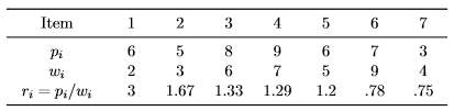
Intuitively, it makes sense to select items with low weight and high profit for the knapsack. To facilitate the picking, we can compute the ratio ri of profit to weight for each item. When proceeding in a greedy fashion, we first pick the item with the highest ri, then the second highest, and so on, until the constraint is met. According to this method, the solution consists of the items {1,2,7}, yielding a total profit of Σ7i=1 xipi = 14 and a total weight of Σ7i=1 xiwi = 9. Let us now consider how we can use a SGA to solve this knapsack problem, by executing the following R code:
library(GA) # Version 3.0.1

# Define data
p <- c(6, 5, 8, 9, 6, 7, 3) # Profits
w <- c(2, 3, 6, 7, 5, 9, 4) # Weights
W <- 9 # Knapsack ’s capacity
n <- length(p) # Number of items

# Define fitness function
knapsack <- function(x) {
  f <- sum(x * p)
  penalty <- sum(w) * abs(sum(x * w) - W)
  f - penalty
}

# Run SGA
SGA <- ga(type="binary",
  fitness=knapsack ,
  nBits=n,
  maxiter=100, # Maximum number of generations
  run=200,     # Stop if the best-so-far fitness
               # hasn't improved for 'run' generations
  popSize=100,
  seed=101)

x.star <- SGA@solution # Final solution: c(1, 0, 0, 1, 0, 0, 0)
sum(x.star)     # Total number of selected items: 2
sum(x.star * p) # Total profit of selected items: 15
sum(x.star * w) # Total weight of selected items: 9
The solution found by the SGA is x∗ = (1,0,0,1,0,0,0), meaning that, under the knapsack’s capacity constraint of W = 9, the optimal solution is to pick the items {1,4} which yields a total profit of f(x∗) = 15. Thus, with the SGA solution we obtain a higher profit than with the greedy approach, although the total weight of selected items is in both cases equal to 9. The reason for the inferiority of the greedy approach is that it performs a local optimization in which the final solution depends on the choices made along the way, and thus got trapped in a local optimum. On the other hand, the SGA only evaluates the fitness of solutions once they are completely constructed. This ultimately allows the SGA to avoid getting trapped in a local optimum and, given enough search time, performs a global optimization.
In this example, we use a brute-force approach to find x∗, and although it is sufficient for this simple example, note that the algorithmic design can further be modified to run more efficiently in finding the global solution. That is, the presented setup does not check whether a newly created solution is also feasible (i.e., not violating the capacity constraint). In order to do so, one could implement an additional mechanism that “repairs” infeasible solutions before fitness evaluation [2, 3]. However, as pointed out by Scrucca [3], the repairing step is unlikely to be computationally very efficient.
The knapsack problem might appear very theoretical, but in fact has diverse practical applications, e.g., in cargo loading, project selection, assembly line balancing, and so on [2]. This problem, however, has also striking similarities with the feature selection task in a data modeling context. That is, the knapsack problem can be parsed into a feature selection problem where the ones and zeros in x represent the inclusion or exclusion of a feature in the model, n is the number of features, the fitness function might consist of the model performance such as the negative Akaike information criterion (AIC) or the negative Bayesian information criterion (BIC), and the constraint on the knapsack’s capacity is—for simplicity—disabled (i.e., W = ∞). Note that lower values of AIC or BIC typically indicate better model performance. This is why these values would need to be multiplied with minus one in order to formulate a maximization problem. Once this has been set up, the x∗ found by the SGA would then indicate the important features. Again, the major advantage of using SGA is that they optimize globally, revealing the optimal set of features that should be included in the analytical model to get the globally best model performance. Compare this, for example, to a stepwise regression model, which includes or excludes features at each step in a greedy fashion—similarly, as illustrated in the simple knapsack problem above. Thus, it is likely that such a greedy procedure gets trapped in a local optimum, especially if the number of features is large.
In conclusion, GAs are powerful meta-algorithms inspired by natural selection that can be used for solving complex optimization problems. Here, we only discussed the application to one instance of constrained optimization: the knapsack problem. In a simple example, we demonstrated that the SGA solution yields a higher total profit than the greedy approach, where both solutions exhibit the same total weight at the capacity limit. Last but not least, we briefly outlined how the knapsack problem can be adapted to a feature selection problem in which a SGA can be utilized to find the globally best set of features.
References
- E. Eiben and J. E. Smith, Introduction to Evolutionary Computing. SpringerVerlag, 2003.
- Yu and M. Gen, Introduction to Evolutionary Algorithms, ser. Decision Engineering. Springer, 2010.
- Scrucca, “GA: A package for genetic algorithms in R,” Journal of Statistical Software, vol. 53, no. 4, pp. 1–37, 2013.