
Contributed by: Eugen Stripling, Seppe vanden Broucke, Bart Baesens
This article first appeared in Data Science Briefings, the DataMiningApps newsletter. Subscribe now for free if you want to be the first to receive our feature articles, or follow us @DataMiningApps. Do you also wish to contribute to Data Science Briefings? Shoot us an e-mail over at briefings@dataminingapps.com and let’s get in touch!
In this column, we demonstrate the Bayesian method to estimate the parameters of the simple linear regression (SLR) model. The goal of the SLR is to find a straight line that describes the linear relationship between the metric response variable Y and the metric predictor X. In the frequentist (or classical) approach, the normal error regression model is defined as follows [1]:
Yi = β0 + β1Xi + εi (1)
where:
- Yi is the observed response of observation i,
- Xi is the level of the predictor variable of observation i, a known constant,
- β0 is the intercept parameter,
- β1 is the slope parameter,
- and εi are independent normal distributions with zero mean and constant variance σ2, N(0,σ2), for i = 1,…,n.
The response Yi of observation i is the sum of two components [1]: (i) the constant term β0+β1Xi and (ii) the random term εi. Due to the induced randomness of εi, Y becomes a random variable as well. In other words, there is a probability distribution of the response variable Y for each level of the predictor variable X, and the means of these probability distributions vary in some systematic fashion with X [1]. The figure below illustrates an example taken from [1] in which it is assumed that the intercept and the slope are known, i.e., β0 = 9.5 and β1 = 2.1.
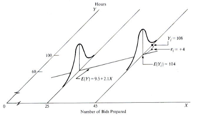
Simple linear regression [1].
Suppose we are in the possession of a data set (X1,Y1),…,(Xn,Yn), where Xi and Yi (i = 1,…,n) are the observed predictor and response measurements of observation i, respectively. We are then able to estimate the model parameters from the data. Usually, our primary interest is in the slope, β1, which reveals how Y will, on average, change when X increases by one unit.
Knowing the value of the slope reveals the strength of the dependency of Y on X. The SLR in fact has a closed-form solution, meaning that the intercept and slope estimates can be computed directly from the data without having to rely on numeric optimization techniques. However, the frequentist approach will return only one solution which is referred to as a single point estimate.
In contrast, as we will see by the end of the column, the Bayesian approach returns a whole distribution of so-called credible values for each parameter. Credibility is a term used to express our belief in certain parameter values. Typically, common probability distributions are used to specify the allocation of credibility over possible parameter values. The benefit of working with distributions is that they provide a natural way to reflect uncertainty of estimates. The application of Bayesian estimation requires a probabilistic reformulation of the SLR, which may look like the following (2):
Yi ∼N(µi,σ)
µi = β0 + β1Xi
β0 ∼N(M0,T0)
β1 ∼N(M1,T1)
σ ∼|Cauchy(G)|
A graphical (perhaps more intuitive) way to represent the same model is achieved by means of Kruschke’s DBDA-style diagrams [2, 3, 4]:
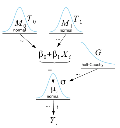
Probabilistic formulation of the simple linear regression model.
From the diagram, it is easy to see that the response Yi of observation i is modeled as a normal distribution with mean µi = β0 + β1Xi and standard deviation σ (depending on the software program, either variance, standard deviation, or precision is specified). To make Bayesian estimation possible, we are required to assign so-called prior distributions to all model parameters, thus making our assumptions about the parameters explicit. In the figure above, we assign for each regression parameter βj (j = 0,1) a normal distribution with mean Mj and precision Tj (reciprocal of the variance), and for σ we assign a half-Cauchy distribution (i.e., considering only non-negative values) with scale parameter G. The prior distributions reflect our prior belief about each parameter in the SLR. If no prior knowledge is available, values for Mj, Tj, and G are typically chosen such that these distributions become so flat that they almost resemble a uniform distribution, implying that we do not favor any particular parameter values.
Additionally, we need to specify an appropriate likelihood, which is the normal likelihood function for the SLR. The likelihood component is the part that incorporates the data. Now, Bayes’ rule [5] can be applied in order to update the priors to the posterior distributions, which reflect the distribution of credible parameter values taken into account the data. When specifying such “weak” priors as described above, even a modest amount of data will easily overrule the priors and the likelihood component will have a much stronger influence on the resulting posterior distributions [3, 4].
To provide a formal definition, suppose we are interested in the estimation of some parameter θ and we are given some data D, Bayes’ rule is then defined as follows [4], (3):
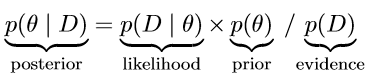
Without going into much detail, the crucial part to remember is that Bayes’ rule merely describes the mathematical relation between the prior and the posterior conditional on the data. In other words, Bayes’ rule precisely dictates how prior allocation of credibility is to be re-allocated to obtain the distribution of credible parameter values taking the data into account [4].
In practice, we typically rely on so-called Markov chain Monte Carlo (MCMC) methods which allow users to generate a large, representative sample from the posterior distribution, which is often also referred to as trace or MCMC chain. Common computer programs to generate such sample are BUGS [6], WinBUGS [7], JAGS [8], Stan [9], and PyMC3 [10]. This sample of representative, posterior parameter values can be utilized to perform statistical inference. In case of the SLR, each step in the MCMC chain, which typically encompasses several thousands, refers to credible parameter values that correspond to estimates for the intercept β0, slope β1, and standard deviation σ. Thus, the Bayesian method returns a whole distribution of credible regression lines. Let us demonstrate the frequentist and Bayesian approach on some toy data. To do so, we assume the true values of the regression parameters are as follows: β0 = 9.5, β1 = 2.1, and σ = 3. Having created the data set, we can now compute the parameter estimates according to the frequentist approach and plot the result (figure below). Clearly, since we estimate the parameter values based on a finite sample of modest size, the estimates will most likely not be exactly equal to the true parameter values. The main message, however, is that the frequentist approach returns only one solution, and therefore no particular notion that accounts for the uncertainty in the parameter estimates is considered.
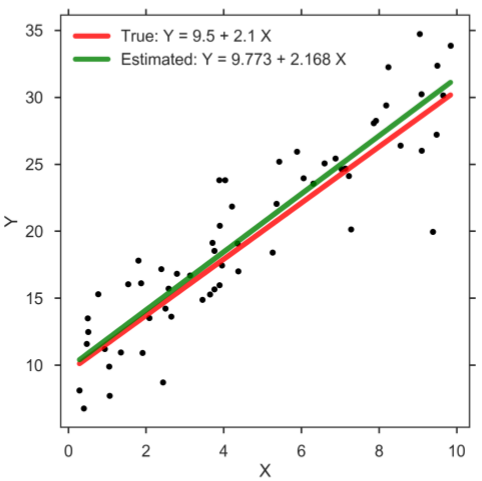
Simple linear regression.
However, when doing data analysis, it can be beneficial to take the estimation uncertainties into account. This can be achieved with Bayesian estimation methods in which the posterior holds the distribution of credible parameter values, which in turn allows user to make a richer statistical inference [3, 4]. When running the computer program, the Bayesian method returns a distribution of credible regression lines (figure below). The figure shows only a sample of credible regression lines randomly taken from the generated MCMC chain. Yet, it can clearly be seen that there is some variation among the lines, reflecting the uncertainty in the parameter estimates.
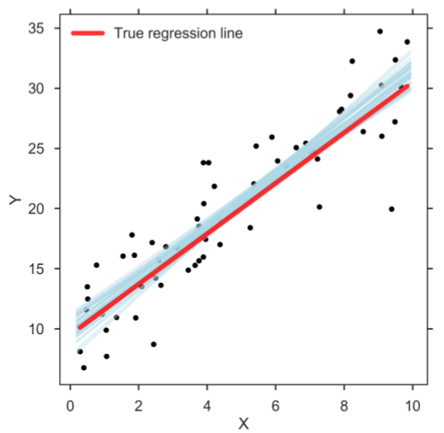
Bayesian SLR: Sample of credible linear regression lines (light blue).
A closer look at the posteriors gives more information about distribution of credible parameter values (figure below). In the figure, the middle numbers correspond to the means computed based on the values in the MCMC chain. The numbers on the left and right are the limits of the 95% highest posterior density (HPD) interval, which corresponds to the minimum width Bayesian credible interval (BCI). Kruschke [3, 4] refers to the HPD as the highest density interval (HDI). Regardless of the terminology, the interpretation is that all values within the 95% HPD are deemed as having the highest credibility. For all three regression parameters, we see that the 95% HPD indeed covers well the true parameter values: β0 = 9.5, β1 = 2.1, and σ = 3:
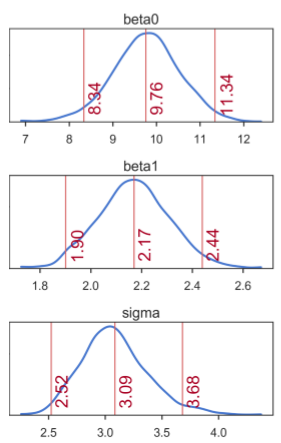
Marginal posterior distributions of each SLR model parameter. Means correspond to the middle numbers. Limits of the 95% HPD interval correspond to the numbers left and right.
Whenever we want to make a prediction of Y given a value of the predictor X (be it the mean or predicted response), we simply go over the MCMC chain and at each step of the chain we plug in the posterior estimates into the regression model to compute the response of interest. In this way, we can create a credible distribution of the mean and predicted response of Y and determine, for example, the 95% HPD (figure below). And indeed, the band for the mean response (darker blue) captures the true regression line well. Similarly, the prediction band (lighter blue) contains almost all observations. Confirming that the Bayesian SLR is a good representation of the data:
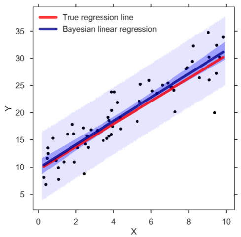
Bayesian SLR with 95% HPD bands for the mean and predicted response. The blue, thick line corresponds to the means of the posterior distributions.
What makes Bayesian methods so attractive is that it is fairly straightforward to adapt the model to challenging circumstances. For example, one could replace the bottom normal distribution in the Kruschke’s DBDA-style diagram figure above, which models the response, with a Student’s t-distribution and rerun the computer program (with some minor adjustments). This modification will make the model robust against outlying observations. Kruschke [4] provides a detailed example of the robust linear regression model. Needless to say, another benefit of Bayesian methods is that they easily allow users to incorporate their valuable expert knowledge into the modeling process by adapting the priors appropriately.
Conclusion
In this column, we demonstrated the application of Bayesian parameter estimation for the simple linear regression model. We showed that the concepts applied in Bayesian inference differ fundamentally from the traditional ones. That is, in the frequentist approach, it is assumed that the data are randomly sampled from normal distributions with fixed parameters. On the contrary, the Bayesian approach assumes the exact opposite, i.e., the data are fixed and the parameters follow some (probability) distribution. Refer to Eq. (3) which expresses the posterior distribution, p(θ | D), of some parameter θ given the data D. Once the data are observed, they are fixed and know to us. It is the set of parameters we are uncertain about and want to learn their true values. In this sense, Bayesian methods are more aligned with circumstances experienced in everyday practice. On top, working with the posterior distribution allows for a richer statistical inference, since more information is processed.
References:
- M. H. Kutner, C. J. Nachtsheim, J. Neter, and W. Li, Applied Linear Statistical Models, ser. McGrwaHill International Edition. McGraw-Hill Irwin, 2005.
- J. K. Kruschke, “Diagrams for hierarchical models – we need your opinion,” [Online; accessed May 2017], 2013.
- Doing Bayesian Data Analysis: A Tutorial with R and BUGS. Academic Press, 2011.
- Doing Bayesian Data Analysis: A Tutorial with R, JAGS, and Stan, 2nd ed. Academic Press, 2014.
- T. Bayes and R. Price, “An essay towards solving a problem in the doctrine of chances. By the late Rev. Mr. Bayes, F.R.S. Communicated by Mr. Price, in a letter to John Canton, A.M.F.R.S.” Philosophical Transactions, vol. 53, pp. 370–418, 1763.
- D. Lunn, C. Jackson, N. Best, A. Thomas, and D. Spiegelhalter, The BUGS Book: A Practical Introduction to Bayesian Analysis, ser. Chapman & Hall/CRC Texts in Statistical Science. Taylor & Francis, 2012.
- D. J. Lunn, A. Thomas, N. Best, and D. Spiegelhalter, “WinBUGS: A Bayesian modelling framework: concepts, structure, and extensibility,” Statistics and Computing, vol. 10, no. 4, pp. 325–337, 2000.
- M. Plummer, “JAGS: A Program for Analysis of Bayesian Graphical Models Using Gibbs Sampling,” in Proceedings of the 3rd International Workshop on Distributed Statistical Computing, 2003.
- Stan Development Team, “The Stan C++ Library, Version 2.15.0.” [Online]. Available: http://mc-stan.org
- J. Salvatier, T. V. Wiecki, and C. Fonnesbeck, “Probabilistic programming in Python using PyMC3,” PeerJ Computer Science, vol. 2, p. e55, 2016. [Online]. Available: https://doi.org/10.7717/peerj-cs.55