
Contributed by: Eugen Stripling, Seppe vanden Broucke, Bart Baesens
This article first appeared in Data Science Briefings, the DataMiningApps newsletter. Subscribe now for free if you want to be the first to receive our feature articles, or follow us @DataMiningApps. Do you also wish to contribute to Data Science Briefings? Shoot us an e-mail over at briefings@dataminingapps.com and let’s get in touch!
A frequently occurring task in data analytic research involves the statistically testing of two learning algorithms. In this column, we showcase the usage of the Bayesian hierarchical correlated t test, a recently proposed statistical method for the comparison of two classifiers on multiple data sets through Bayesian hierarchical modeling [1, 2]. In particular, we demonstrate its application by means of an example in which we compare two well-known machine learning algorithms on churn data.
Example: kNN versus AdaBoost
Suppose that we are given q = 5 churn data sets and we are interested in comparing the two classifiers: k-nearest neighbors (kNN) and AdaBoost. Our task is to determine whether there is a significant difference between the two learning algorithms based on their classification performance measured on all data sets. If there is a difference, also determine which of the two is the better performing classifier. For measuring the classification performance, we use the area under the ROC curve (AUC) metric. To conduct the statistical test, we also need to specify the region of practical equivalence (ROPE), which is a small interval such that any value within the ROPE is equivalent to the value of interest for all practical purposes [1, 3]. Corani et al. [1] proposed to consider two classifiers to be practically equivalent when their performance difference belongs to the interval (−0.01,0.01). The ROPE is a very useful concept for statistical testing that is commonly applied in Bayesian analysis. Ultimately, it allows computing the posterior probabilities of two classifiers being practically equivalent or significantly different [1].
In the next step, we execute 10 runs of stratified 10-fold cross-validation for each classifier on all data sets. It is thereby important to make sure that the same folds are used for both classifiers. This procedure gives us n = 10 × 10 = 100 AUC estimates for each classifier on each data set. The differences of AUC on each fold of cross-validation can then be computed, which are denoted as xi = {xi1,xi2,…,xin} with i = 1, …, q. The values xi = {xi1,xi2,…,xin} are correlated due to the overlapping training sets created in the cross-validation procedure. The Bayesian hierarchical correlated t test corrects for the correlation in an adequate manner. Interested readers are referred to [1] for the technical details of the correction.
The Bayesian Hierarchical Model
Let δi and σi respectively be the actual mean difference between the two classifiers and the standard deviation on the i-th data set. Formally, the Bayesian hierarchical model is defined as follows [1]:
| xi ∼ MV N(1δi,Σi), | (1) |
| δ1,…,δq ∼ t(δ0,σ0,ν), | (2) |
| σ1,…,σq ∼ unif(0,σ¯). | (3) |
Priors for the parameters of the high-level distribution:
| δ0 ∼ unif(−1,1), | (4) |
| σ0 ∼ unif(0,σ¯0), | (5) |
| ν ∼ Gamma(α,β), | (6) |
| α ∼ unif(α,α¯), | (7) |
| β ∼ unif(β,β¯). | (8) |
In Eq. (1), it is assumed that the cross-validation values xi = {xi1,xi2,…,xin} of the i-th data set are generated from a multivariate normal whose components have the same mean (δi), the same standard deviation (σi), and correlation (ρ). The value of ρ is estimated to be the reciprocal of the number of folds used in cross-validation (in our example: ρ = 1/10). Thus, each diagonal element of the covariance matrix Σi equals σi2 and each off-diagonal element equals ρσi2. Notice that in this formulation each data set i is modeled to have its own mean δi and standard deviation σi, allowing to express the location and uncertainty of the mean difference.
Further, it is assumed that the δi’s are drawn from a high-level Student’s t distribution with mean δ0, scale factor σ0, and degrees of freedom ν (Eq. (2)). The t distribution allows for accommodating outliers since it is more flexible than the Gaussian, and it is therefore a common choice for robust Bayesian estimation [1, 3]. Ultimately, our primary interest lies in the estimation of δ0. The quantity δ0 expresses the average difference in performance between the two classifiers on the population of data sets. Eq. (2) models the dependency of the mean differences in the single data sets (δi’s) on δ0. Modeling this relationship as a hierarchical dependency gives rise to the so-called “shrinkage effect.” In short, when jointly estimating the δi’s, it shifts (or shrinks) the estimates toward each other, making the estimates more conservative. Because of this, shrinkage yields a lower estimation error than the traditional approach, as Corani et al. [1] also proved formally. To estimate a quantity with Bayesian methods, one has to assign a prior distribution to it. For δ0, it is assumed to be uniformly distributed within −1 and 1 (Eq. (4)). This is a reasonable choice for all performance measures bounded within ±1 such as AUC, accuracy, recall, or precision.
The quantity δ0 only specifies the location of the t distribution. It is also necessary to estimate the scale parameter (σ0), a quantity to express uncertainty, as well as the degrees of freedom (ν) to fully specify the t distribution. The degrees of freedom can be thought of as a parameter that expresses the resemblance to a normal distribution. This is, if ν > 30, the t distribution is practically a normal and when ν < 30 it is a heavy tailed distribution, suitable for dealing with outliers. To estimate these parameters, one has to assign prior distributions to them as well (Eq. (5) – (8)). In particular, note that for ν, a Gamma distribution is assigned, and a Uniform prior to both of its parameters α and β. In this way, the parameter values for α and β are simultaneously estimated in the inference process, and one does not have to specify any fixed values for them. Uniform priors are also assigned to estimate the standard deviation of each data set (Eq. (3)). Much more can be said about the choices made for each prior and its parameters. For more details, we refer the interested reader to [1]. In any case, users of the test can feel reassured that the specifications of the priors are well-justified in research literature.
The Bayesian hierarchical correlated t test applies a Markov-Chain Monte Carlo sampling method to obtained representative samples from the posterior distribution, which form the foundation for performing statistical inference and drawing conclusions. To do so, the probabilistic programming language Stan [4], a language for Bayesian inference, is used to generate a representative sample from the posterior.
To conduct the statistical test, we stack together the n = 100 differences of AUC obtained on each of the q = 5 churn data sets into a q × n matrix. This matrix is used as an input for the Bayesian hierarchical correlated t test.
Test Result
The outcome of the test can be visualized by means of a probability simplex (Figure 1). It can be seen that most of the posterior mass is in the region in favor of AdaBoost, which is the region at the right bottom of the triangle corresponding to the case where AdaBoost is more probable than kNN and ROPE together. Visualizing the posterior mass in this way has the additional benefit of getting a sense of the estimation uncertainty.
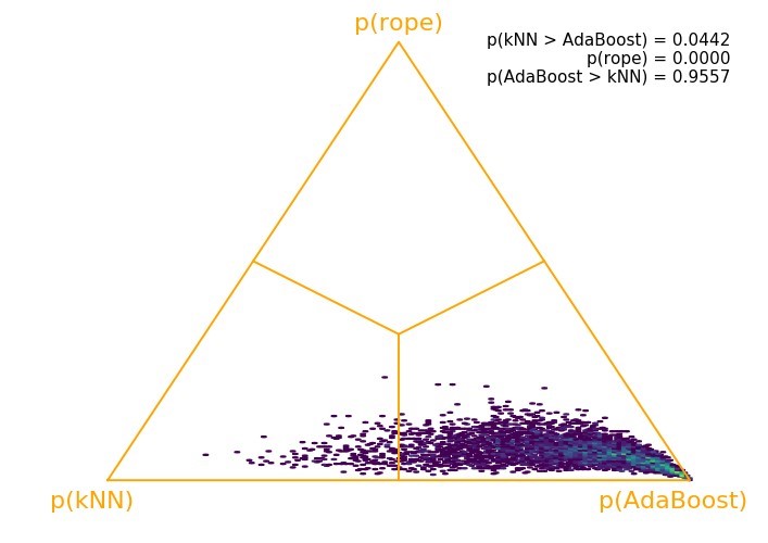
Figure 1: Posterior of kNN versus AdaBoost based on differences of AUC for all five churn data sets.
As a hard rule, Corani et al. [1] proposed to use a probability cut-off value of 95% to declare significance. Given that p(AdaBoost > kNN) = 0.9557, we can conclude that AdaBoost is practically better than kNN with a probability of approximately 96%. “Practically better” means that AdaBoost is superior to kNN—not only in terms of statistical significance—but also in terms of having a higher practical impact.
In the event that none of the three probabilities exceeds the 95% threshold, Corani et al. [1] proposed to make use of the posterior odds: o(left,right) = p(left)/p(right). In our example, p(left) and p(right) would correspond to p(kNN > AdaBoost) and p(AdaBoost > kNN), respectively. Thus, posterior odds larger (smaller) than 1 indicate that there is evidence in favor of left (right). Corani et al. [1] proposed the following grades of evidence:
| Posterior odds | Evidence |
| 1-3 | weak |
| 3-20 | positive |
| > 20 | strong |
In any case, the Bayesian hierarchical correlated t test allows users to draw meaningful conclusions, regardless whether or not the test result is significant. Unlike with conventional statistical methods, a major advantage of using the Bayesian hierarchical correlated t test is that it allows for testing whether the two classifiers in question are practically equivalent. In such case most of the posterior mass would lie in the upper region of the triangle and we would conclude that the difference in performance between the two classifiers has no practical significance.
In conclusion, the Bayesian hierarchical correlated t test is an adequate statistical method for testing two classifiers on multiple data sets. The hierarchical model applied in the test jointly analyzes the cross-validation results of the two classifiers. Thanks to the hierarchical structure, this gives rise to the shrinkage effect, resulting in more accurate estimates than with the traditional approach. This method equips researchers not only to test for statistical significance, but—more importantly—to test whether the difference between two classifiers has a practical impact! Moreover, the test allows computing the probabilities that are of real interest to researchers, namely for example: What is the probability of classifier 1 performing better than classifier 2, given the data? Knowledge of these probabilities allows for better decision making. Even in the case of an insignificant test result, the Bayesian hierarchical correlated t test still makes it possible for users to draw a meaningful conclusion—a desirable property for any statistical test!
References
- Giorgio Corani, Alessio Benavoli, Janez Demšar, Francesca Mangili, and Marco Zaffalon. Statistical Comparison of Classifiers Through Bayesian Hierarchical Modelling. Machine Learning, pages 1–21, 2017.
- Alessio Benavoli, Giorgio Corani, Janez Demšar, and Marco Zaffalon. Time for a Change: a Tutorial for Comparing Multiple Classifiers Through Bayesian Analysis. arXiv preprint arXiv:1606.04316, 2017.
- John K. Kruschke. Bayesian Estimation Supersedes the t Journal of Experimental Psychology: General, 142(2):573–605, 2013.
- Bob Carpenter, Andrew Gelman, Matthew D. Hoffman, Daniel Lee, Ben Goodrich, Michael Betancourt, Michael A. Brubaker, Jiqiang Guo, Peter Li, and Allen Riddell. Stan: a Probabilistic Programming Language. Journal of Statistical Software, 76(1):1–32, 2017.