Forgetting the Past to Learn the Future: Long Short-Term Memory Neural Networks for Time Series Prediction

Long Short-Term Memory neural networks (LSTM’s) are a type of recurrent neural networks that has been used for many state-of-the-art applications in recent years, such as speech recognition, machine translation, handwriting recognition and, of course, time series prediction. Originally, Hochreiter and Schmidhuber¹ conceived LSTM’s as a solution to the ‘vanishing gradient problem’, which refers to the rapid decay in influence of past values on the output. Long-term dependencies were therefore difficult to model with, for example, simple recurrent neural networks. This ability of LSTM’s to handle a much larger context, is precisely what makes them so interesting for any application where dependencies are crucial, such as natural language and time series analysis. In this column, we will explain how the fundamentals of LSTM’s work and how to pre-process time series data as input for this type of recurrent neural network.

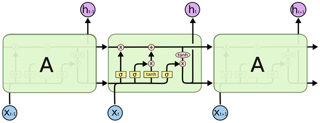
The fundamental idea behind LSTM’s is combining recurrent neural networks with a memory aspect that naturally selects which information to remember and which information to regret. In order to achieve this goal, every LSTM unit consists of three or four elements, or ‘gates’. Each gate computes a value between 0 and 1 that refers to how much of the information should pass through that gate. In the figure below², each layer of the LSTM block consists of a yellow rectangle, which communicates with the horizontal line on the top that represents the cell state. The first gate on the left is the ‘forget’ gate, which produces a decision about which parts of the previous information to keep in the memory. The next yellow element constitutes the ‘input’ layer, which decides which elements should be updated with new information, while the third element creates a list of new information that could be added to the memory. When we put these two layers together, it becomes clear which values should be replaced in the cell state. The results of these three layers are then used to update the cell state by forgetting what should be forgotten according to the first layer, and by updating the information that needed to be replaced according to the second and third layers. Finally, the fourth layer consist of the ‘output’ gate, which selects the elements that should actually be outputted by the entire block. LSTM blocks can be used recurrently after one another or can be inserted into other neural network structures.

Now that we understand the fundamentals of LSTM’s, we can turn to the times series data itself. When pre-processing time series for neural networks, we need to transform the data into a correct input format for the LSTM. Firstly, the time series needs to be stationary, as neural networks perform the best when predicting the variance that cannot be contributed to any seasonal or trend component³. Therefore, we can, for example, apply differencing and/or seasonal differencing on the data beforehand, depending on the data’s characteristics. Secondly, the entire time series should be normalized, as the LSTM expects the data to be in the same scale as the activation function, such as, for example, the hyperbolic tangent. The output of the LSTM will have to undergo the opposite process of these two steps in order to reflect the true predicted value for the time series. Finally, the data needs to be adjusted to look like a supervised learning dataset, i.e. a continuous label is linked to a set of variables. This label is the value of the time series at time t + 1, while the variables consist of the values of time series until time T. The number of previous time steps to include in the model, is a hyper parameter that requires attention. Generally, more training data is better, but this parameter can be determined by a validation set in order to ensure the best fit with the given data. These steps assume a one-step-ahead prediction, but larger prediction horizons are possible as well. The neural network can either be trained to have multiple outputs or the LSTM with one-step-ahead prediction can take previously predicted values as new input.

In short, LSTM’s are a popular form of neural networks that can take on many different applications. Generally, the more long-term dependencies are present in the data, the better LSTM’s perform. Applications involving language, both written and spoken, and time series are therefore a perfect fit with this type of recurrent neural network. In forecasting, LSTM’s have been especially useful in applications with frequent time periods, such as load forecasting and traffic forecasting. In these cases, the LSTM certainly benefits from the large number of data points to train on.

References:

• Hochreiter, Sepp, and Jürgen Schmidhuber. “Long short-term memory.”Neural computation 8 (1997): 1735-1780.
• Christopher Olah. Understanding LSTM Networks. Github blog, 27 Aug. 2015, http://colah.github.io/posts/2015-08-Understanding-LSTMs/. Accessed 12 June 2017.
• Zhang, G. Peter, and Min Qi. “Neural network forecasting for seasonal and trend time series.”European journal of operational research 2 (2005): 501-514.