
Contributed by: Seppe vanden Broucke
This article first appeared in Data Science Briefings, the DataMiningApps newsletter. Subscribe now for free if you want to be the first to receive our feature articles, or follow us @DataMiningApps. Do you also wish to contribute to Data Science Briefings? Shoot us an e-mail over at briefings@dataminingapps.com and let’s get in touch!
Various classification settings suffer from a high degree of class imbalance. For instance, in the setting of customer churn, it is very likely that the number of non-churners heavily outweigh the number of churners. This poses a challenging environment for standard supervised classification techniques. Since most techniques inherently optimize towards accuracy (or another loss definition which is balanced according to the class frequencies), they will inherently be more sensitive to detecting the majority class. If we don’t take care of the issue, the classification output will be biased towards the majority class — in some cases even by simply always predicting the majority class. This is a sensible default choice. E.g. assuming a training data set contains 99% non-churners, the majority of classifiers would have a hard time improving on the 99% accuracy rate by simply classifying all instances as a non-churner.
Nevertheless, in settings like these, this is not really what we want a classifier to do. Given that the minority class is commonly the positive class of interest in many settings (e.g. a churner, a defaulter, a rare disease), we need to look for ways to have our classifier look towards identifying such cases. Obviously, this will come at a cost of making more errors with regards to false positives (i.e. we will also mis-classify negative cases as positive), though this is a price we’re willing to pay. The question will hence be which approach will lead to the highest recall (identifying minority positive cases) whilst keeping precision at a satisfactory rate as well.
Several approaches exist to encode this concern into a classification pipe line:
- The majority of methods work on the data level, meaning that the training data is pre-process in such a way that the balance between the minority and majority class is re-adjusted. Two simple methods to do so include randomly oversampling (duplicating) instances belonging to the minority class, or randomly undersampling (removing) instances beloning to the majority class, until the desired ratio is obtained.
- Other techniques work on the algorithm level, meaning that the training data is kept as is but the classification technique is modified to work better with imbalanced data sets. Common approaches include cost-sensitive learners (setting different costs and benefits on the four outcomes of a binary confusion matrix), instance weighting (where e.g. the minority instances are given a higher weight), changing the loss function for approaches that support it (e.g. see [1]), or modifying existing techniques, e.g. by modifying the bootstrap procedure for random forests to provide balanced batches [2].
Throughout the past, various “smart sampling” techniques have been proposed that try to perform either under- or oversampling in a manner which is more intelligent and uses the inherent structure of the data. For oversampling, two well known approaches include SMOTE (Synthetic Minority Oversampling Technique, [3]) and ADASYN (Adaptive Synthetic, [4]). Both of these techniques create new, synthetic minority instances by interpolating between existing instances, rather than simply duplicating instances in place:
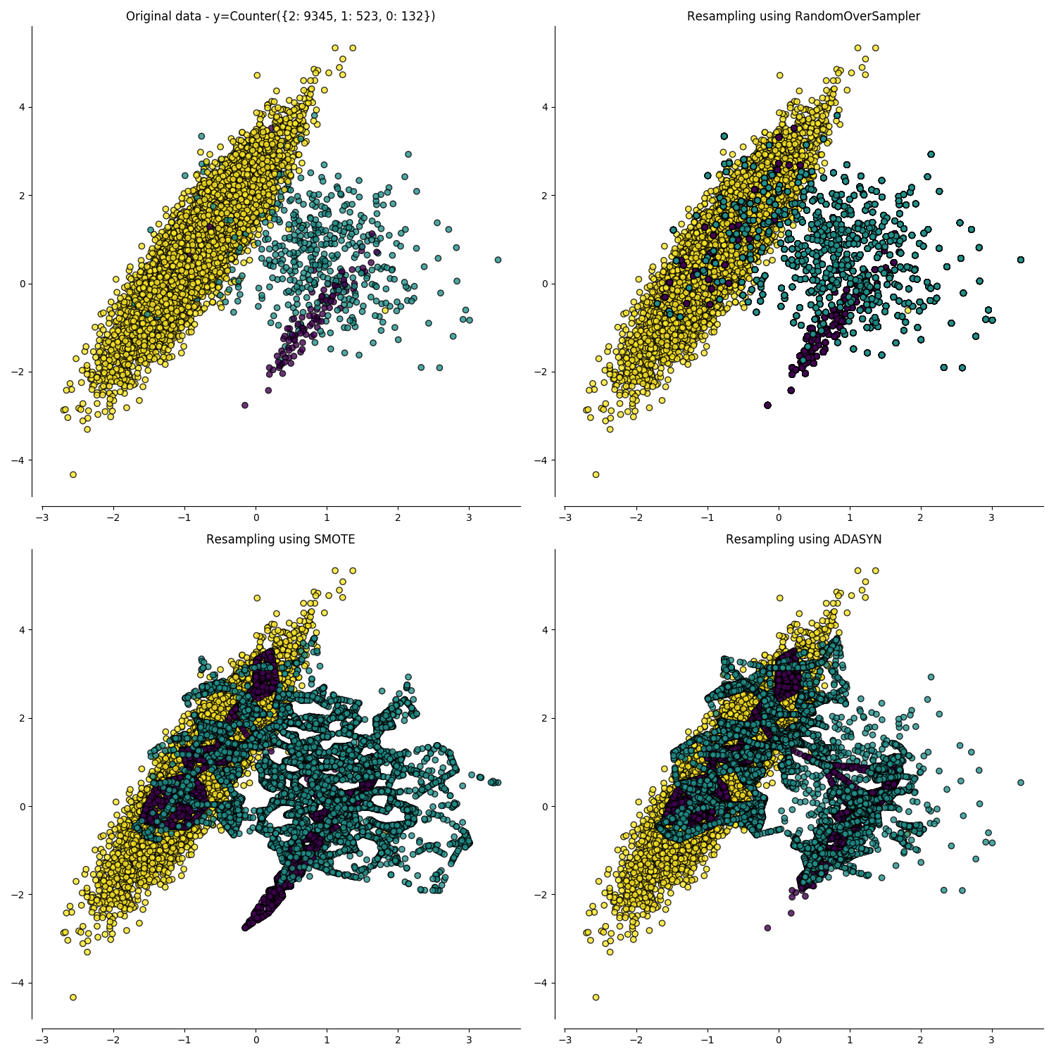
SMOTE and ADASYN (example taken from https://imbalanced-learn.readthedocs.io/en/stable/over_sampling.html)
In some cases, the greedy interpolation strategy adopted by these techniques can lead to the creation of new instances which add in noise by creating instances which overlap with the majority instances, making the subsequent classification more difficult. As such, follow-up extensions like Borderline-SMOTE aim to fix this problem by avoiding creating instances that are close to majority cases [5,6].
Similarly, also for under-sampling techniques, a number of extensions have been proposed, most of which are based on removing majority instances when it can be observed that they do not add much information, for instance because they’re densely surrounded by many other majority instances. As such, common approaches involve a clustering technique, use nearest neighbors, or Tomek links [7] (a Tomek link describes two instances of opposing class that are each other’s nearest neighbor).
Tuning sampling approaches
Data-driven approaches to rectify imbalanced data sets can involve quite a bit of guesswork. That is, it is commonly not clear whether the usage of more advanced sampling techniques will work better than the naïeve random based approaches. Similarly, no real guidelines exist with regards to the ratio to resample towards, other than trying several values or sticking to a sensible 50:50 ratio, i.e. biasing the classifier to consider both classes as being equally important a-priori.
Let us take a look at a real-life example to show the effect of these parameters in practice. To do so, we will utilize the churn data set from this Kaggle competition, together with the imbalanced learn Python package, which implements a large number of sampling based techniques.
data = pd.read_csv('https://raw.githubusercontent.com/Macuyiko/' +
    'mlc-churn/master/WA_Fn-UseC_-Telco-Customer-Churn.csv', index_col=0)
data.Churn.describe()
data.Churn[data.Churn == 'Yes'].count() / data.Churn.count()
data.Churn[data.Churn == 'Yes'].count() / data.Churn[data.Churn == 'No'].count()
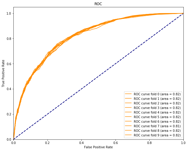
Investigating the data set reveals 7043 total samples with 27% churners and an a-priori minority/majority class ratio of 0.36. This is not an extreme class imbalance, so let us first see how a classifier performs on the unbalanced data. We first preprocess the data and create train and test splits. Next, we train a random forest on 10 folds over the train data set:
X_train, X_test, y_train, y_test = train_test_split(data.loc[:, data.columns != 'Churn'], data.Churn,
test_size=0.33, stratify=data.Churn)
clf = RandomForestClassifier(n_estimators=100)
plt.figure()
plt.xlim([0.0, 1.0])
plt.ylim([0.0, 1.05])
plt.xlabel('False Positive Rate')
plt.ylabel('True Positive Rate')
plt.title('ROC')
plt.plot([0, 1], [0, 1], color='navy', lw=lw, linestyle='--')
folder = StratifiedKFold(n_splits=10)
for k, (train_index, val_index) in enumerate(folder.split(X_train, y_train)):
    clf.fit(X_train, y_train)
    tpr, fpr, thresholds = roc_curve(y_test, clf.predict_proba(X_test)[:, 1])
    plt.plot(tpr, fpr, color='darkorange', label='ROC curve fold %s (area = %0.2f)' % (k, auc(tpr, fpr)))
plt.legend(loc="lower right")
plt.show()
Next, we iterate over a number of under- and oversampling techniques and different sampling rations (positive; minority / negative; majority). As our evaluation metric, we will use AUC, again over a 10-fold CV:
techniques_to_consider = [
    RandomUnderSampler,
    RandomOverSampler, SMOTE, ADASYN, BorderlineSMOTE, SVMSMOTE,
]

ratios_to_consider = np.arange(0.10, 3, 0.1)
folder = StratifiedKFold(n_splits=10)
classifier = RandomForestClassifier(n_estimators=100)
evaluator = lambda tr, sc: roc_auc_score(tr, sc)

def get_resample_dict(y, ratio, change_pos=True):
    y_incl_pos, y_incl_neg = sum(y == 1), sum(y == 0)
    assert y_incl_pos <= y_incl_neg
    if change_pos:
        return { 0: y_incl_neg, 1: np.ceil(ratio * y_incl_neg).astype(int) }
    else:
        return { 0: np.ceil(y_incl_pos / ratio).astype(int), 1: y_incl_pos }

def get_resampled(X_include, y_include, ratio, technique):
    resample_pos = lambda y : get_resample_dict(y, ratio, True)
    resample_neg = lambda y : get_resample_dict(y, ratio, False)
    with warnings.catch_warnings():
        warnings.simplefilter("ignore")
        try:
            technique_instance = technique(sampling_strategy=resample_pos)
            X_resampled, y_resampled = technique_instance.fit_resample(X_include, y_include)
        except ValueError:
            try:
                technique_instance = technique(sampling_strategy=resample_neg)
                X_resampled, y_resampled = technique_instance.fit_resample(X_include, y_include)
            except ValueError:
                return None, None
    return X_resampled, y_resampled

results = []
for technique in tqdm_notebook(techniques_to_consider):
    print(technique)
    for ratio in tqdm_notebook(ratios_to_consider):
        folds_info = []
        for k, (train_index, val_index) in enumerate(folder.split(X_train, y_train)):
            X_include, X_validation = X_train.iloc[train_index], X_train.iloc[val_index]
            y_include, y_validation = y_train.iloc[train_index], y_train.iloc[val_index]
            X_resampled, y_resampled = get_resampled(X_include, y_include, ratio, technique)
            if X_resampled is None:
                continue
            classifier.fit(X_resampled, y_resampled)
            scores = classifier.predict_proba(X_validation)[:, 1]
            evaluation = evaluator(y_validation, scores)
            folds_info.append( (k, evaluation, resample_dict) )
        results.append( (technique.__name__, ratio, np.mean([r[1] for r in folds_info]), folds_info) )
Next, we plot the results for each technique:
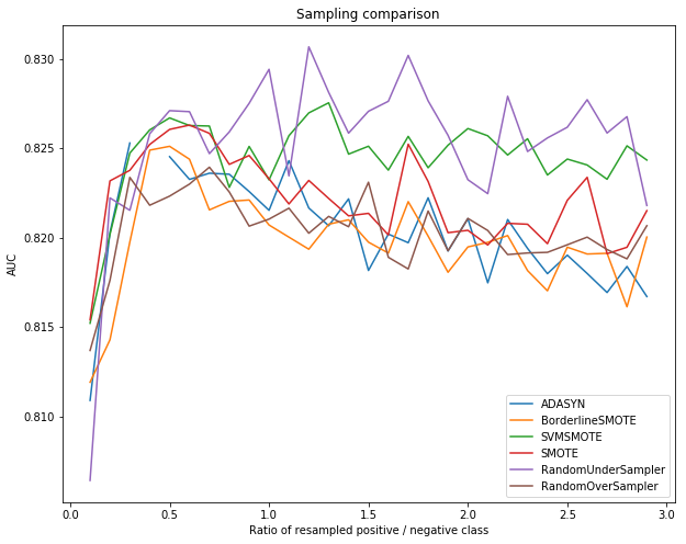 Based on this, we can observe the following:
- Random undersampling performs well and better than various advanced techniques
- The setting of the ratio has an impact. 0.5 turns out to be a good value for this data set
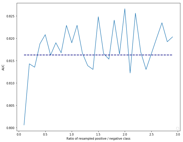
Based on these results, it appears that smart sampling techniques do not significantly outperform random sampling approaches. Let us compare random undersampling over the left-out test set (the dotted line represents the unbalanced AUC result):
 One might argue that AUC is not always the best metric to utilize when tuning sampling approaches for imbalanced learning. Indeed, it is important to tune and decide on a sampling approach based on your metric of interest, such as top-decile lift. In 2017, together with prof. Bing Zhu, we contrasted and evaluated several sampling approaches on a large number of churn data sets. From which the following take-aways were concluded:
- Depending on the metric and classification technique used, different sampling strategies will behave differently. Sampling has little influence on logistic regression, for instance, but vary when using tree based techniques.
- Random undersampling and oversampling stand out as being good default choices in most settings, confirming the finding above that more smart sampling techniques do not commonly offer significant improvements.
- The commonly utilized “default” sampling rate of 1:1 might not be the best option given your data set and metric. It is hence important to carefully tune the sampling ratio on your data set and evaluation metric as outlined above.
References
- [1]: Wang, S., Liu, W., Wu, J., Cao, L., Meng, Q., & Kennedy, P. J. (2016, July). Training deep neural networks on imbalanced data sets. In 2016 international joint conference on neural networks (IJCNN) (pp. 4368-4374). IEEE.
- [2]: Chen, Chao, Andy Liaw, and Leo Breiman. “Using random forest to learn imbalanced data.” University of California, Berkeley 110 (2004): 1-12.
- [3]: N. V. Chawla, K. W. Bowyer, L. O.Hall, W. P. Kegelmeyer, “SMOTE: synthetic minority over-sampling technique,” Journal of artificial intelligence research, 321-357, 2002.
- [4]: He, Haibo, Yang Bai, Edwardo A. Garcia, and Shutao Li. “ADASYN: Adaptive synthetic sampling approach for imbalanced learning,” In IEEE International Joint Conference on Neural Networks (IEEE World Congress on Computational Intelligence), pp. 1322-1328, 2008.
- [5]: H. Han, W. Wen-Yuan, M. Bing-Huan, “Borderline-SMOTE: a new over-sampling method in imbalanced data sets learning,” Advances in intelligent computing, 878-887, 2005.
- [6]: H. M. Nguyen, E. W. Cooper, K. Kamei, “Borderline over-sampling for imbalanced data classification,” International Journal of Knowledge Engineering and Soft Data Paradigms, 3(1), pp.4-21, 2009.
- [7]: I. Tomek, “Two modifications of CNN,” In Systems, Man, and Cybernetics, IEEE Transactions on, vol. 6, pp 769-772, 2010.