
Contributed by: Jeroen Frans
This article first appeared in Data Science Briefings, the DataMiningApps newsletter. Subscribe now for free if you want to be the first to receive our feature articles, or follow us @DataMiningApps. Do you also wish to contribute to Data Science Briefings? Shoot us an e-mail over at briefings@dataminingapps.com and let’s get in touch!
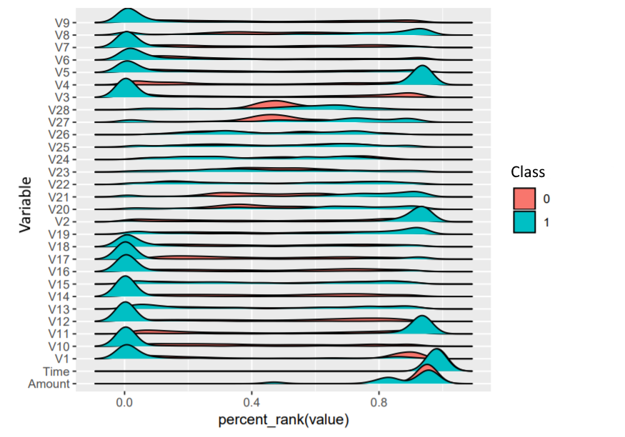
For this demonstration of using autoencoders in the context of fraud detection, we’ll use a Kaggle data set that is readily available. It contains European credit card transactions in the period of September 2013. Note that fraud is a rare phenomenon: out of the total of 284,807 transactions only a mere 492 were fraudulent. This corresponds to an incidence rate of 0.172%. This means there is a strong class imbalance. The dataset contains 28 numerical features (V1 – V28) that are the result of a PCA transformation (for confidentiality reasons). On top of these features also the time is registered (expressed as seconds after the first observation) as well as the transaction
A visual inspection of the data already shows that some of the features have a different distribution for the fraudulent cases compared to the non-fraudulent ones:
As preparatory steps, we take the (chronologically) first 230,000 data points as a training set and the rest for validation. This resembles the real-life scenario where you will want to predict for future transactions whether they are fraudulent based on the earlier transactions done.
df <- read_csv("Data/creditcard.csv", col_types = list(Time = col_number()))
df_train <- df %>% filter(row_number(Time) <= 230000) %>% select(-Time)
df_test <- df %>% filter(row_number(Time) > 230000) %>% select(-Time)
## Picking joint bandwidth of 0.0309
We are going to use autoencoders to detect the fraudulent cases. To do so, we will only use the non-fraudulent training data to learn an encoding function for the data. When we apply this on the validation set, we expect to see that the fraudulent transactions are not well reconstructed and can hence be detected. Since an autoencoder is a type of neural network, it is very important to normalize your data first. You can do this by rescaling the data to either a [0,1] or [-1,1] range or by standardizing them so that they are normally distributed with mean 0 and standard deviation 1. In R we can use the caret package which has a preprocessing functionality. With this functionality, we create a transformator with our training data that we can apply on the “future” data points or test set.
minMaxScale <- df_train %>% select(-Class) %>%
  preProcess(method = "range")
  # use c("center", "scale") for standardization
x_train <- predict(minMaxScale, df_train) %>%
  select(-Class) %>%
  as.matrix() #You need this format for tensorflow to accept it as input
x_test <- predict(minMaxScale, df_test) %>%
  select(-Class) %>%
  as.matrix()
y_train <- df_train$Class
y_test <- df_test$Class
Next, we need to design a neural network model architecture. In this example we will use Keras to define our model architecture and Tensorflow to do the actual calculations. Here we will use three hidden layers. One with 12 neurons, one bottleneck layer of 6 and one layer of 12 again. For the activation function we will use the hyperbolic tangent function. Any non-linear function should work fine here and you can also use linear functions. You can play around with other activation functions like ReLU and sigmoid as well. If you were to use an identity function as activation, then the autoencoder would perform similar to a PCA analysis.
Also, since we are training on only the non-fraudulent transactions, you will want to learn as much as possible from these transaction. We can also consider increasing the number of nodes in the symmetric hidden layers to a number higher than 28. This will make the model learn latent features in the data and puts less emphasis on compressing the data. We did not use Time as a feature in the model. A great possible way to further improve the model could be by engineering a new feature out of this variable.
After having defined the model, we compile it and train it. The loss function used is the mean squared error. This makes sense since we want to minimize the distance between our inputs and the reconstructed output. For the optimization, adam was used.
model <- keras_model_sequential()
model %>%
  layer_dense(units = 12, activation = "tanh", input_shape = ncol(x_train)) %>%
  layer_dense(units = 6, activation = "tanh") %>%
  layer_dense(units = 12, activation = "tanh") %>%
  layer_dense(units = ncol(x_train))
summary(model)
model %>% compile(
  loss = "mean_squared_error",
  optimizer = "adam"
)
history <- model %>% fit(
  x = x_train[y_train == 0,],
  y = x_train[y_train == 0,],
  epochs = 30,
  batch_size = 256,
  validation_data = list(x_test[y_test == 0,], x_test[y_test == 0,])
)
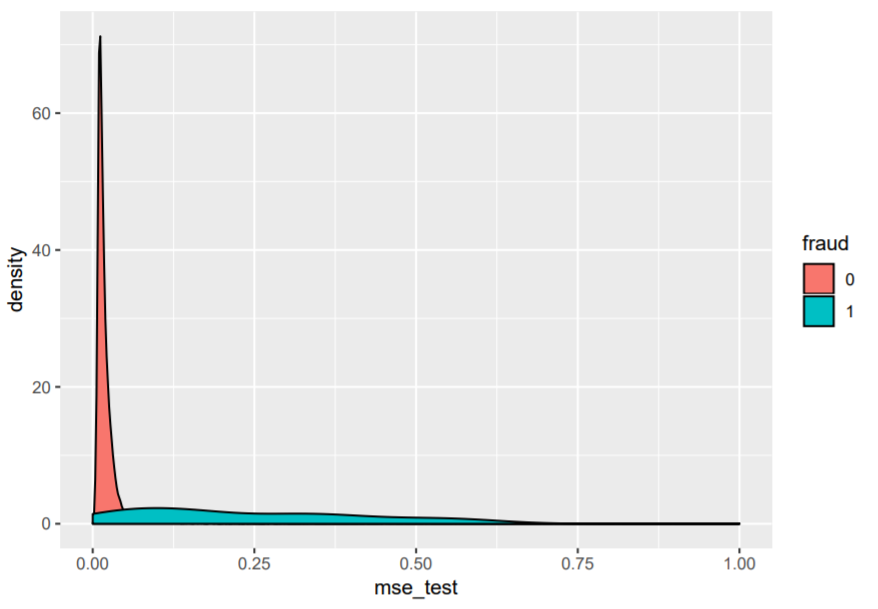
If we now look at the reconstruction error (MSE) on the test set we see that there are some quite extreme outliers. Most errors lie between 0.01 and 0.025, but there are larger cases going up to 14. The density plot also shows the difference in reconstruction error between non-fraudulent transactions (in red) and fraud (in blue). We can see that there is a different distribution in terms of reconstruction error:
pred_train <- predict(model, x_train)
mse_train <- apply((x_train - pred_train)^2, 1, sum)
pred_test <- predict(model, x_test)
mse_test <- apply((x_test - pred_test)^2, 1, sum)
The way we handle this outcome might depend on the resources that are available. One very coarse approach is to take the 200/500/. . . observations with the highest reconstruction error of our test set or perhaps the 0.1% with highest reconstruction error. A second approach is to find a good cutoff value based on precision, recall or other evaluation measures. A third approach is to find a cost-optimal cutoff value. This means we will have to express the cost of investigating a transaction, the cost of a fraud case that goes undetected and possibly also the cost of a false alarm. Let’s try the first approach:
top_200 <- plotdata %>% arrange(desc(mse_test)) %>% top_n(200)
## Selecting by mse_test
incidence_rate <- sum(top_200$y_test)/200
We see that in the 200 highest there is an incidence rate of 19%. Compared to the dataset as a whole, which had an incidence rate of fraud of 0.17%, this is already quite an improvement.
The second approach would be to create a tradeoff based on precision and recall values of the model:
possible_k <- seq(0, 1, length.out = 100)
precision <- sapply(possible_k, function(k) {
  predicted_class <- as.numeric(mse_test > k)
  sum(predicted_class == 1 & y_test == 1)/sum(predicted_class)
})
ggplot(data=as.data.frame(cbind(possible_k,precision)), aes(x = possible_k, y = precision)) +
geom_line(color="steelblue") + xlab("k treshold")
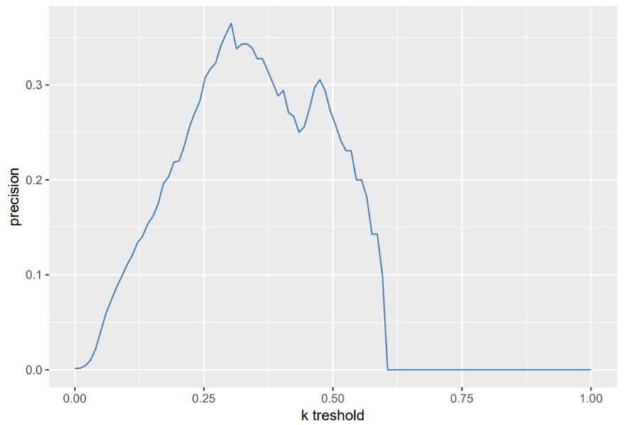
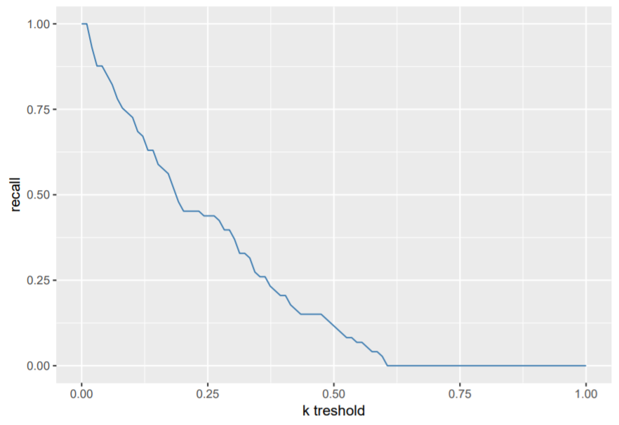
We want to detect as many fraud cases as possible, but try to avoid false alarm cases. If we merely look at the precision, we see that the optimal cutoff is somewhere around 0.3. Be aware however, that you also have to balance it out with respect to other evaluation measures like the recall value.
recall <- sapply(possible_k, function(k) {
  predicted_class <- as.numeric(mse_test > k)
  sum(predicted_class == 1 & y_test == 1)/sum(y_test)
})
ggplot(data=as.data.frame(cbind(possible_k,recall)), aes(x = possible_k, y = recall)) +
geom_line(color="steelblue") + xlab("k treshold")
In practice, there might be a cost involved in having wrong predictions. This can change the cutoff problem
to a cost optimisation problem. Every inspection of a transaction could have a fixed cost, since an employee
will have to spend time on it. Suppose this cost is 2.5 euro. The cost of not detecting a fraud case will also
have a cost, namely the amount of money of the fraudulent transaction. The problem would then change to:
avg_cost_per_check <- 2.5
lost_money <- sapply(possible_k, function(k) {
  predicted_class <- as.numeric(mse_test > k)
  sum(avg_cost_per_check * predicted_class + (predicted_class == 0) * y_test * df_test$Amount)
})
ggplot(data = as.data.frame(cbind(possible_k,lost_money)), aes(x = possible_k, y = lost_money)) +
geom_line(color="steelblue") + xlab("k treshold") + ylab("Cost")
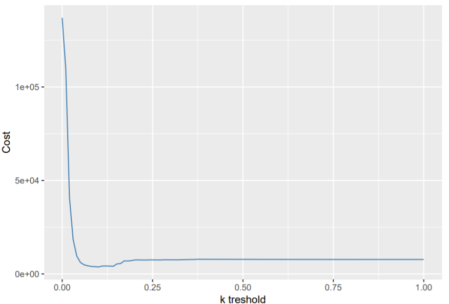
Now the optimal cutoff would be 0.101. You could also make the cost function more complex: there might also be a cost for false
alarms, where y_test == 0 and predicted_class == 1. Customers could leave when their card is blocked too often for no reason. What would be the cost of losing a customer?
This initial exploration and some of the cost functions are inspired on a blog post of D Falbel, which includes an extra section on hyperparameter tuning. The workflow would look very similar in Python: the model is trained with the same Tensorflow/Keras setup and the normalization can be done with scikit-learn. Code for this post can be found on this Gitlab repository.