
This article first appeared in Data Science Briefings, the DataMiningApps newsletter. Subscribe now for free if you want to be the first to receive our feature articles, or follow us @DataMiningApps. Do you also wish to contribute to Data Science Briefings? Shoot us an e-mail over at briefings@dataminingapps.com and let’s get in touch!
Recommender systems have been defined by Shapira et al already in 2011 as software tools and techniques providing suggestions for items to be of use to a user. Two key concepts here are items and users. As a simple example think of items as books on Amazon and users as readers. Recommender systems typically start from a rating matrix like the one shown below.
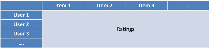
A rating matrix is constructed by aggregating user interest data into a single user item score per user and item pair. The rows represent the users the columns represent the items. The rating then depends upon the observed interest, measured either implicitly or explicitly.
Matrix factorisation or matrix decomposition is commonly used in building recommender systems. The idea is to factorize or decompose the rating matrix into a product of other matrices which provide a more condensed, focused representation of the information in the rating matrix. Put differently, factorization is a way of approximating a matrix when it is prone to dimensionality reduction because of correlations between columns or rows. In its most simple form, we decompose the rating matrix into a user feature matrix and an item feature matrix. The features can then disclose interesting characteristics of the data. Note that these features are sometimes also referred to as concepts or latent factors.
The idea of singular value decomposition or SVD is to decompose the rating matrix R in the unique product of 3 matrices. The aim is to reveal latent factors in the rating matrix R by minimizing the Root Mean Squared Error (RMSE).
Before we get into the details of SVD, let’s first refresh some matrix basics. The rank of a matrix is the maximum number of columns or rows that are linearly independent. Consider the matrix shown below.
[ 2  4  8
  1  2  3
  4  8  2
  4  8  0 ]
As you can see, the third row equals the sum of the first and fourth row minus two times the second row. Likewise, the second column equals two times the first column. Hence, the rank of this matrix is 2. Also remember that an N times N square matrix whose rank is less than N is not invertible and is also called singular. If a matrix has rank r, then SVD will decompose it into matrices whose shared dimension is r. Vectors are called orthogonal if their dot product equals 0. Consider the two vectors shown below.
[1, 4, 6].[2, -2, 1]t=1 × 2 + 4 × (-2) + 6 × 1 = 0
You can clearly see that their dot product equals 1×2+4x(-2)+6×1 which equals 0. Hence, both vectors are orthogonal, which also implies that they are linearly independent. A unit vector is a vector with norm 1. Remember, the norm, sometimes also called the Frobenius norm, is the square root of the sum of the squares. For the below vector, this becomes 1/5 + 4/5 or 1.
[ 1/sqrt(5) 2/sqrt(5) ]
Finally, an orthonormal basis is a set of unit vectors that are pairwise orthogonal.
After this refresher of basic matrix concepts, we are now ready to introduce singular value decomposition or SVD. You can see it illustrated below.
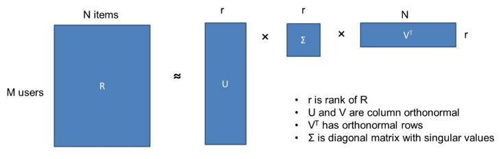
We start from the M by N rating matrix R for M users and N items. We decompose it into the product of 3 matrices. U is an M by r matrix. Σ is a square r by r matrix. VT is an r by N matrix. r is the rank of the rating matrix R. U and V are column orthonormal. VT has orthonormal rows. Σ is a diagonal matrix with the singular values along the diagonal. As said, Σ is an r × r diagonal matrix with the singular values. Some of these singular values will be exactly 0 depending upon the rank of the rating matrix R. Typically, there will be some big singular values and some smaller ones. The aim of SVD is now to make r smaller by setting the smallest singular values to 0 since these are assumed to correspond to noise. The effect of this is that it renders the corresponding columns of U and V useless which results into a more compact representation. You can see this illustrated below.
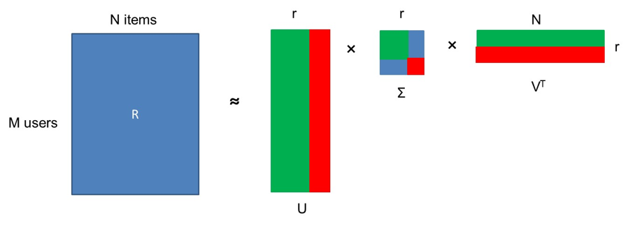
Let’s first look at the Σ matrix with the singular values. Suppose the singular values in the red square are low and the ones in the green square high. If we set the singular values in the red square to 0, then you can see that the red columns in U become useless. Likewise, the red rows in VT become useless. This will result into a more compact approximation of the rating matrix R.
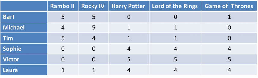
Let’s work out an example to illustrate how SVD works. Suppose we have a rating matrix, as shown above, with 6 users: Bart, Michael, Tim, Sophie, Victor and Laura. We have 5 movies Rambo II, Rocky IV, Harry Potter, Lord of the Rings and Game of Thrones. Since it’s a small rating matrix, we can make some quick observations. Bart, Michael and Tim especially like action movies, such as Rambo II and Rocky IV, and are not fond of fantasy movies such as Harry Potter, Lord of the Rings and Game of Thrones. Sophie, Victor and Laura don’t like action movies, but they do like fantasy movies. You can see that the Harry Potter and Lord of the Rings columns contain identical values, so the rank of this matrix is 4.
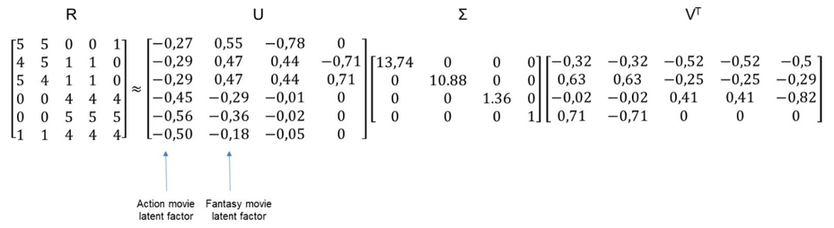
Above you can see the result of the SVD decomposition. Let’s look at the diagonal Σ matrix in the middle first. You can see it’s a 4 by 4 square matrix and not a 5 by 5 square matrix. The reason is because the rank of the rating matrix R was 4, so one of the singular values turned out to be 0 and was dropped. You can see it has two big singular values 13,74 and 10,88 and two smaller ones 1.36 and 1. This indicates that there are two latent factors in the rating matrix. Let’s look at the first two columns of the U matrix. In the first column, you can see a distinction between the first three values and the last three. Essentially, this models the action movie latent factor liked by Bart, Michael and Tim. Let’s look at the second column of the U matrix now. Again, you see a discrepancy between the first 3 values and the final 3 values. This essentially models the fantasy movie latent factor concept, as liked by Sophie, Victor and Laura. Essentially, the matrix U can be interpreted as a user to latent factor similarity matrix. The singular value 13.74 represents the strength of the action movie latent factor concept, whereas the singular value 10.88 indicates the strength of the fantasy movie latent factor concept. Finally, the V matrix can be interpreted as the movie to latent factor similarity matrix. Let’s look at its first two rows. In the first row, you can see a distinction between the first two values and the final three values. This corresponds to the action movie latent factor concept. Let’s now look at the second row. You can see a discrepancy between the first two values and the final three values. This corresponds to the fantasy movie latent factor concept. We are now ready to do dimensionality reduction. We will put the two smallest singular values 1.36 and 1 to zero, or reduce the Σ matrix to a 2 by 2 matrix. Obviously, this will remove the corresponding columns from the U and V matrices.
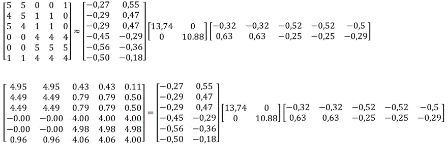
Above you can see the result of this. We now have a two by two Σ matrix with only the 2 biggest singular values corresponding to the 2 latent factors we identified earlier. Let’s now also figure out how good this approximation is. At the bottom, we calculated the exact dot product of the U, Σ and VT matrices. You can see that the result approximates our original rating matrix pretty good. The difference between both the original matrix and the approximation can be quantified using the root mean squared error, RMSE, or Frobenius norm of the differences.
An obvious question when doing SVD is to pick the right amount of singular values or r. This can be done using the concept of energy, which is defined as the sum of the squares of the singular values. Let’s reconsider our earlier Σ matrix.
[  13.74   0   0   0
    0  10.88   0   0
    0     0 1.360  0
    0     0    0   1  ]
The energy is calculated as 13.74²+10.88²+1.36²+1² which gives 310. A common rule of thumb then states that we choose r such that the retained singular values keep at least 90% of the energy. In other words, if we drop 1.36 and 1, the resulting energy is 307 such that we managed to keep 99% of the energy.
Singular Value Decomposition is a very popular dimension reduction technique in building recommender systems. Note that the winning entry for the famous Netflix Prize used a number of SVD implementations and optimised variants thereof. SVD is also frequently used in text analytics to reduce the dimensionality of the document by term matrix.