
This article first appeared in Data Science Briefings, the DataMiningApps newsletter. Subscribe now for free if you want to be the first to receive our feature articles, or follow us @DataMiningApps. Do you also wish to contribute to Data Science Briefings? Shoot us an e-mail over at briefings@dataminingapps.com and let’s get in touch!
Contributed by: Bart Baesens, Tim Verdonck
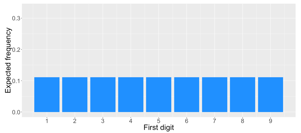
In this article, we’ll introduce Benford’s law, which describes a surprising and fascinating fact about the distribution of the first digits of numbers. We’ll explain how this law has become an important tool in detecting fraud. Let’s start by taking a newspaper at a random page and write down the first or leftmost digit which is either 1, 2, 3, until 9. What are the expected frequencies of these digits? If all digits are equally likely then we expect to observe each digit as the first digit in approximately 1 out of 9 or 11% of cases as shown below.
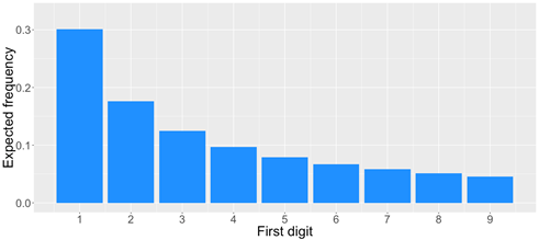
Benford’s law, however, predicts a different distribution for the first digit of a number. According to Benford’s law, the probability that the first digit equals 1 is about 30%, while it’s only 4.6% for digit 9.
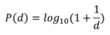
This surprising phenomenon was first discovered by astronomist Newcomb in 1881 and later rediscovered by Benford in 1938. Both noted that in a book of logarithms the first pages, with low first digits, are more frequently used than the last pages with digits 7, 8 and 9 since they were more dirty. In that time logarithm tables were frequently used to speed up the multiplication of two numbers. Benford analyzed the distribution of the first digits in 20 tables concerning populations, molecular weights, mathematical sequences and death rates. In total he observed 20,229 numbers by hand. He found the leading digit, d=1 to 9, occurs with a probability:
The antifraud rationale behind the use of the law is that producing empirical distributions of digits that conform to the law is difficult for non-experts. Fraudsters may thus be biased toward simpler and more intuitive distributions, such as the uniform. Strong deviations from the expected frequencies might indicate that the data is suspicious, possibly manipulated, and thus fraudulent. Hence, Benford’s law can be used as a screening tool for fraud detection. If Benford’s law is not satisfied, then it is probable that the involved data was manipulated and further investigation is required. Conversely, if a data set complies with Benford’s law, it can still be fraudulent. Data sets satisfying one of the following conditions typically conform to Benford’s Law.
- Data where numbers represent sizes of facts or events
- Data in which numbers have no relationship to each other
- Data sets that grow exponentially or arise from multiplicative fluctuations
- Mixtures of different data sets
- And finally, some well-known infinite integer sequences
Typically, the more orders of magnitude that the data covers (at least 4 digits) and the more observations we have (typically 1000 or more), the more likely the data set will satisfy Benford’s Law.
We have already seen that many real datasets conform to Benford’s Law. Most financial data and accounting numbers generally conform to Benford’s Law. Fraudsters typically change the dataset by adding invented numbers or changing real observations which do not follow Benford’s Law. Due to these abnormal duplications and atypical numbers, the dataset is not conform to Benford’s Law anymore. Hence Benford’s Law is a popular tool for fraud detection since it identifies deviations that need further review. It is even legally admissible as evidence in the US in criminal cases at the federal, state and local levels. Benford’s law has been successfully used for
- check fraud
- electricity theft
- forensic accounting
- payments fraud
Benford’s Law was for example used as evidence of voter fraud in the 2009 Iranian election. Mark Nigrini showed that Benford’s Law could be used in forensic accounting and auditing as an indicator of accounting and expenses fraud.
Not every dataset has to conform to Benford’s Law and many will never do. Examples are:
- If there is a lower and/or upper bound or data is concentrated in a narrow interval, e.g. hourly wage rate or height of people.
- If numbers are used as identification numbers or labels, e.g. social security number, flight numbers, car license plate numbers, phone numbers.
- If fluctuations are additive instead of multiplicative, e.g. heartbeats on a given day
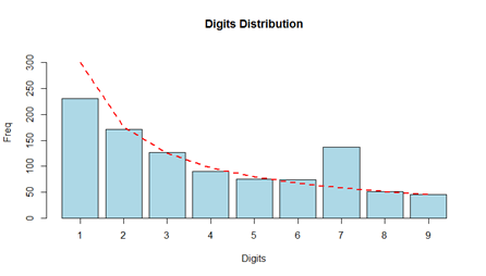
Let’s work out an example of using Benford’s law for fraud detection. Assume the internal audit department of a company needs to check employee reimbursements for fraud. Employees may reimburse business meals and travel expenses after mailing scanned images of receipts. Assume we want to analyze the amounts that were reimbursed to employee Tom in the last 5 years. Below you can see the distribution of the reimbursements depicted by the light blue histogram. The red line corresponds to Benford’s law. It is clear that the dataset has less 1’s and more 7’s than expected under Benford’s Law. Based on this discrepancy, the company can then further investigate Tom’s expenses. After analyzing his reimbursements starting with 7, it was detected that Tom replaced 1/3 of his expenses starting with a 1 by a 7 before scanning the receipt.
Benford’s law has also been extended to the first-two digits. A dataset satisfies Benford’s Law for the first-two digits if the probability that the first-two digits equal is approximately:
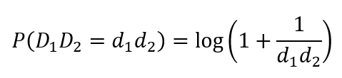
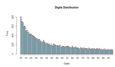
This test is considered more reliable than the first digits test and is more frequently used in fraud detection. Below you can see an example of this. This data contains the populations of 19509 towns and cities of US (July 2009). You can see that the distribution of the first two digits nicely corresponds to Benford’s law.
We can then create predictive features based on Benford’s law. More specifically, we can featurize the discrepancy between the empirical distribution and Benford’s law using a statistical distance measure such as the Kullback-Leibler divergence or Kolmogorov-Smirnov statistic. These can then be added to the fraud data set for predictive modeling.
For more information, we are happy to refer to our BlueCourses course Fraud Analytics.