
This article first appeared in Data Science Briefings, the DataMiningApps newsletter. Subscribe now for free if you want to be the first to receive our feature articles, or follow us @DataMiningApps. Do you also wish to contribute to Data Science Briefings? Shoot us an e-mail over at briefings@dataminingapps.com and let’s get in touch!
This week’s contribution stems from our most recent BlueCourses course Customer Lifetime Value Modeling.
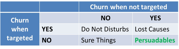
Uplift modeling provides an interesting alternative to churn prediction modeling and setting up well targeted-marketing campaigns. It reformulates the target variable from the ones who are about to churn to the ones who are about to churn and can be retained with a marketing campaign. In other words we want our analytical models to focus on the persuadables that need the campaign to not churn. Let’s look at the below table. We can distinguish between 4 customer segments. The Do Not Disturbs are the customers that will not churn if not targeted, but if targeted feel annoyed and will churn because the marketing campaign has an adverse effect on them. The lost causes are the ones that churn anyway, whether targeted or not. The sure things are the ones that will not churn, even when not targeted. Hence, it’s lost money targeting them. The persuadables are the ones that need the campaign to prevent them from churning. These are the ones we should actually target with our campaign.
In uplift modeling, one makes a distinction between gross and net effect. Gross effect represents all the customers that do not churn. However, it could be that some of these non-churners were not intending to churn anyway and didn’t need the campaign to stay. Net effect represents the customers that do not churn because of the campaign specific effect. Obviously, the uplift perspective to churn prediction introduces bigger complexity since we can never precisely observe the net effect of a treatment. In other words, we cannot simultaneously apply a treatment and not apply a treatment to the same individual. This essentially reduces to a problem of causal inference. Uplift modeling closely relates to prescriptive analytics as it tries to precisely prescribe which customer population we should target using well-designed analytical models.
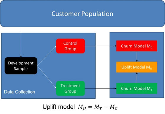
A first and rather straightforward and intuitive approach for developing uplift models is called the Two-model approach, also referred to as the naïve approach, difference score method, or double classifier Approach as illustrated in the above figure. We start by drawing a sample from our entire customer population. We then split this up into control group and a treatment group. The control group is not subject to the marketing retention campaign. The treatment group represent the customers targeted with the retention campaign. Next, we develop a churn model for the control group, Mc, and a churn model for the treatment group, Mt. Both can be developed using any classification technique such as logistic regression, decision trees, etc. The uplift model is then the difference between both as illustrated. In other words, the uplift model estimates the uplift by subtracting the churn probability when not treated, estimated by the Control churn Model, from the churn probability when treated estimated by the Treatment churn Model. It is indirect in the sense that uplift is not directly estimated by a model that is fitted to produce uplift scores. Instead, uplift is calculated indirectly from both estimated churn probabilities. It has the benefit of being straightforward to implement.
A second and more elegant direct approach for uplift modeling makes use of logistic regression and was introduced by Victor Lo in 2002. The proposed methodology groups the Treatment and Control Groups in one development sample and incorporates a treatment dummy variable, which indicates Treatment or Control Group membership.
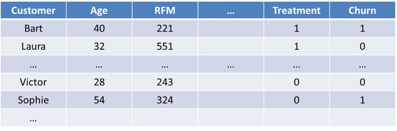
In the example dataset above, the treatment dummy variable is assigned a value of zero for the Control Group and a value of 1 for the Treatment Group. Lo’s approach then includes the treatment indicator, as well as all other variables and all possible interaction terms, as indicated in bold, in the following logistic regression model:
![]()
Obviously, Lo’s method calls for a variable selection procedure to be applied to reduce the number of variables. The interaction terms that are explicitly included in Lo’s method allow the model to account for the heterogeneous effect of a treatment based on the characteristics of a customer, as expressed by the predictor variables. If a treatment works well in a particular segment, for instance significantly decreases the churn rates in the customer segment with age < 30, then including the interaction terms allows the logistic regression model to pick up this pattern in the uplift model and to more accurately predict uplift. In other words, including these interaction terms increases the power of the approach. Usually, interaction terms are not preferred in business applications because of the reduced interpretability of the resulting analytical model. In Lo’s approach however, the interaction terms are less complex because the treatment variable is a simple dummy variable, and the reason for adopting these interaction terms can be quite easily explained to a non-expert. Including these interaction effects allows data scientists and marketeers or campaign developers to gain insight into the possibly divergent effects of a retention campaign across various subgroups in the customer population. By setting up well-designed experiments and by applying customized treatments to different samples of customers, one can customize the campaign characteristics in terms of, for example, channel or incentive, to match the exact customer profile. This allows to further boost the returns on marketing efforts.
When using Lo’s method the uplift effect can be calculated as the difference between the probability when treated (t=1) and probability if not treated (t=0). A key advantage of Lo’s method, when compared to the two-model approach, is that only one model is needed which facilitates its adoption. Also the interaction effects are a key benefit.
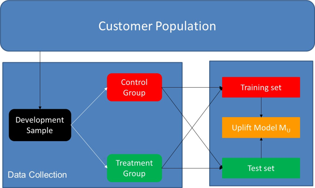
Once we have developed our churn uplift models, we can start evaluating them. Note that the models developed on the control and treatment group, which can either be two classification models, as in the two model approach, or one classification model, as in Lo’s approach, both have a training and test set. To evaluate the performance of the uplift model, we will use the combined test set from the control group and the treatment group. The distribution of treatment and control group customers in the test set is preferably identical to the overall distribution in the development sample and training set to avoid possible sources of bias.
A very interesting visual evaluation approach is to plot the actual churn rate per decile in the combined test set containing both Treatment and Control group observations.
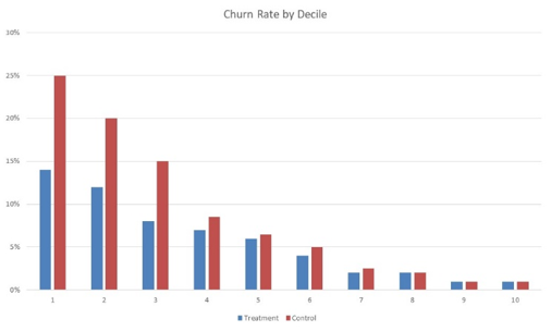
Note that a lower decile corresponds to a higher predicted uplift score as it results from our uplift model. Hence, ideally a higher uplift should be obtained in the first deciles. In other words, the differences in observed churn rates should be bigger. As can be seen from the plot, the churn rate in both treatment and control groups decreases with lower deciles which is intuitively clear. However, what we are actually interested in is the difference between the churn rates in the treatment and control group. Remember that customers in the treatment group were targeted with a retention campaign whereas customers in the Control Group received no campaign. You can see that the uplift if the first 3 deciles is high, which is really nice. Based on this graph, I would personally suggest to target the customers in the first 3 uplift deciles. Note that you can also easily turn the graph into an uplift by decile graph which only plots the uplift by decile.