A Refresher on ANOVA for Multivariate Testing in Web Analytics

Contributed by: Bart Baesens, Seppe vanden Broucke

The idea of multivariate testing is to test more than one element on a page at the same time.  Suppose we have an on-line movie rental store and we need to decide on our home page as you can see illustrated here.

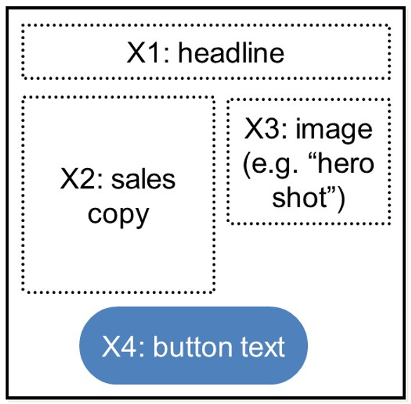
We experiment with 2 choices for the headline: unlimited movies or cheap movies.  This is variable X1.  Variable X2 is the sales copy and say we want to choose between 3 movies.  Variable X3 is an image, or our hero shot, and we want to choose between a male and female actor.  Variable X4 is the button text and here we choose between either “Try it Now” or “Discover”.

Multivariate testing will now try all of these together, or a careful selection thereof, and also see whether there are any interactions.  Essentially, what we do in multivariate testing is design an experiment, so we are going to adopt some statistics terminology.  Every variable has a branching factor which corresponds to the values it can take.  Variables X1, X3 and X4 can take on 2 values, let’s denote these by a and b.  Variable X2 can take on 3 values which we denote by a, b and c.  The variables and their values are also called factors and factor levels. A “recipe” is then a combination of factor levels.  For example, X1a, X2b, X3a, X4b which is also abbreviated as abab.  The search space then consists of all possible recipes, which is simply the product of the branching factors or 24 in our case.

We can construct the recipes in 2 possible ways.  In an unstructured way, any choice of number of variables and their branching factors is possible.  In a structured way, we put restrictions on the choices available.  The data can then be collected using methods borrowed from the field of experimental design.  According to a full factorial experimental design, we generate pages for all possible recipes.  According to a fractional factorial design, we only consider a subset of recipes.  The Taguchi method is a well-known experimental design method that uses orthogonal arrays to obtain maximal information with a relatively small number of recipes.  It enables you to make inferences based on a carefully prescribed selection of possible recipes rather than by randomly sampling from the entire search space of recipes.  Other popular experimental design methods are Plackett–Burman, Latin Squares and choice modelling.

Two types of data analysis can be considered.  In parametric analysis, we try to build an explicit statistical model explaining the effects of the variables on a goal metric.  An example of the latter could be the conversion rate.  In non-parametric analysis, we just try to find the best recipe across the large search space without explaining why it is best.  Popular examples of parametric analysis are regression methods or analysis of variance (ANOVA).  Let’s elaborate a bit further on this.

Analysis of Variance or ANOVA is one of the key underlying techniques to do multivariate testing.  ANOVA is a statistical method to estimate how the mean for an outcome variable, such as the amount spent or conversion rate, depends on one, two or more categorical variables.  One-way ANOVA tests the impact of one categorical variable, such as the type of image (female versus male actor), two way ANOVA tests the impact of two categorical variables such as the impact of an image (male versus female actor) and movie (movie 1, 2 or 3), and multi-way ANOVA tests the impact of 3 or more categorical variables such as image (male versus female actor), movie (movie 1, 2 or 3) and headline (Unlimited Movies or Cheap Movies).  The basic idea of ANOVA is to partition the total variation in the data, measured by the sum of squared deviations into 2 sources: the variation within the groups and the variation between the groups.  Both are then compared to see whether there is a difference or not. In other words, the null hypothesis states that the group means are similar whereas the alternative hypothesis states that the group means are different or

• H₀: group means are similar
• H_A: group means are different

ANOVA relies on a few assumptions.  First of all, it assumes independent groups or in other words, the observations in one group or category are independent of the observations in all other groups or categories. Next, it assumes homogeneity of the variances. The population variances of the outcome variable are the same for all possible categories. Finally, it assumes that there is a sufficiently large sample size for the outcome variable to be normally distributed.  Obviously, this is the assumption that is typically the hardest to satisfy.

Let’s work out an example of two-way ANOVA.  We want to test the impact of a female versus male actor image and 3 movies on the amount spent as you can see in the below table.

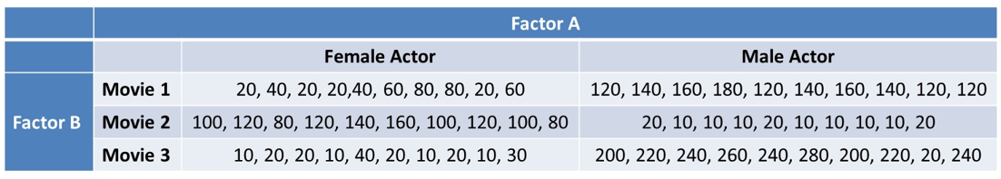
This is an example of a balanced design since we have an equal number of observations in each category, more specifically 10 observations.  We now need to introduce some notation as follows:

• a = number of levels of factor A (e.g., 2)
• b = number of levels of factor B (e.g., 3)
• r = total number of observations per cell (e.g., 10)
• Y_ijk = value of observation k for factor A = i and factor B = j (e.g., Y₂₃₆ = 280)
• bar{Y_…} = overall average across all observations (e.g., 93)
• bar{Y_i..} = average when factor A has value i (e.g., bar{Y_2..} = 127,66)
• bar{Y_.j.} = average when factor B has value j (e.g., bar{Y_.2.} = 62,5)
• bar{Y_ij.} = average when factor A has value i and factor B has value j (e.g., bar{Y_23.} = 230)

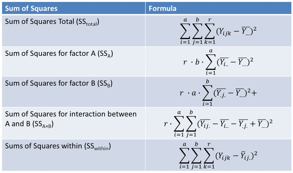
The ANOVA procedure then performs a decomposition of the sum of squares to determine how much variability in the outcome variable is explained by the different categories as follows:

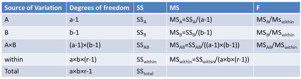
We can now look at the various source of variation, the corresponding degrees of freedom, the sum of squares as defined previously, the mean sum of squares or MS which is simply the sum of squared divided by the degrees of freedom, and then finally the corresponding F statistic which can be used to perform the hypothesis test.

Various software packages can be used to perform ANOVA such as SAS, R, Python, but also Microsoft Excel.  Below we actually just used Microsoft Excel.

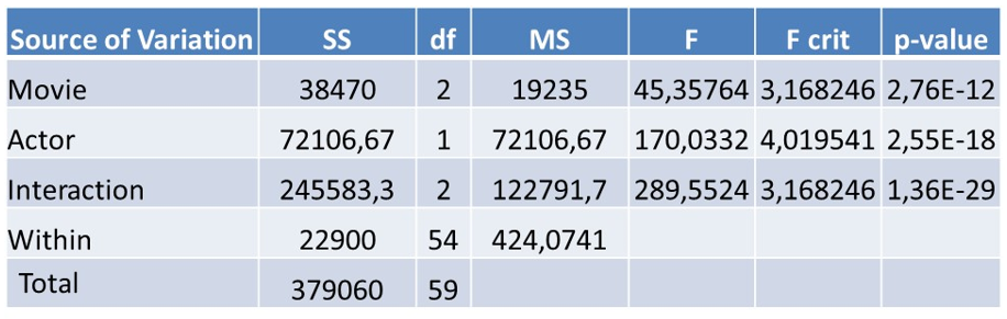
You can see that the analyses for Movie, Actor and Interaction all give very low p-values which indicates that they are all statistically significant.  Various follow-up analyses can then be performed to dig into more detail.  ANOVA can also be easily extended to Multivariate analysis of variance or MANOVA which is simply an ANOVA analysis but now with several dependent variables such as amount spent, Time on Site, etc.

For more information, see our newest BlueCourses course on Web Analytics.