Markov Chains for CLV Modeling: a Review

Contributed by: Bart Baesens, Seppe vanden Broucke

Let’s start with the basic idea of Markov Chains before we work out a small example.  We start from a collection of random variables X₀, X₁, X₂, etc. which can take values in one of M states.

The process is said to be a finite-valued Markov chain if

P(X_t+1=j|X₀=k₀, X₁=k₁, …,X_t-1=k_t-1, X_t=i) = P(X_t+1=j|X_t=i) for all t, i, j where 1 ≤ i and j ≤ M

In other words, once the current state is known, the history may be thrown away.  The current state is a sufficient statistic for the future.  Essentially, a Markov process is a memoryless random process.  The probabilities P(X_t+1=j|X_t=i) are called transition probabilities and are usually represented as p_t(i,j).  Obviously, all probabilities are between 0 and 1 and at any given time point t, the sum of the probabilities of moving from a given state i to any other state j should equal 1.

The transition probabilities can be obtained using the idea of maximum likelihood where the probabilities p(i,j) = n(i,j)/n(i) with n(i) the total number of times state i appeared and n(i,j) the total number of times the sequence (i,j) appeared from time 1 to T.  Note that there are Chi-squared testing procedures available to test for the Markov assumption.  The reason the Markov assumption is often made is because it simplifies simulations as we will see below.  Also, it is an assumption which comes close to reality in many real-life situations.  As an example consider weather forecasting.  If we adopt a very simple model stating the weather of tomorrow is the same as that of today, then you will in fact observe that you have a pretty good weather forecasting model.

Let’s work out an example of Markov Chain analysis in a Customer Lifetime Value (CLV) setting.  Examples of customer states could be platinum, gold, silver, bronze and churn.  Other examples could be based on the outcome of an RFM analysis or deciles of the CLV distribution.  Three types of transitions can be distinguished: staying in the current state, upgrading from silver to gold for example, or downgrading from bronze to churn for example.  Note that in this case churn is considered an absorbing state since once in it, you can not get out of it anymore.

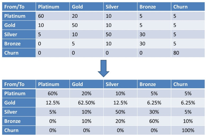
Below you can see an example of a transition matrix with 5 states: platinum, gold, silver, bronze and churn.  You can see the absolute numbers at the top.  At the bottom, you can see the corresponding maximum likelihood probabilities.  Note again that churn is an absorbing state, so once in it, you cannot get out of it anymore.  Hence, the 100% in the lower right cell.

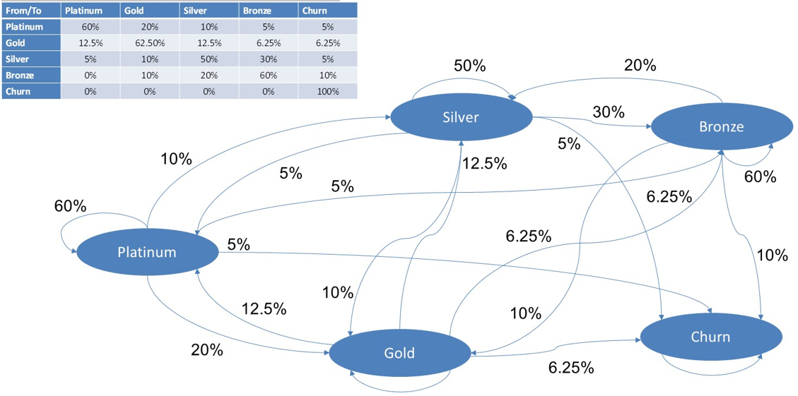
Here you can see an alternative network representation of our Markov Chain.  The nodes represent the states.  The arcs the transitions.  The transition probabilities are added next to each arc.  Obviously, from a given node all transition probabilities should sum to 1.  The more states the harder it becomes to visualize the Markov chain as a network.

Let’s study the migration matrix into some more detail.  As said, all migration probabilities are between 0 and 1 and the sum across the rows is always 1.  The latter is obvious since a customer can either keep the same state, downgrade or upgrade.  Do note that the sum across the columns is not equal to 1.  When smooth transitions are desired, the business might require the transition probabilities to decrease as you are getting further away from the diagonal, so some additional smoothing operators might be applied.  Above diagonal elements represent downgrades and below diagonal elements represent upgrades. Also note that many migration matrices are typically diagonally dominant which means that many customers tend to keep their state and only a minority migrates.  These then typically represent the loyal customers with a steady-state purchasing behavior.

Remember the Markov assumption which stated that the state at time t+1 only depends upon the state at time t.  Because of this assumption, it is really easy to start doing simulations or projections by multiplying the transition matrix by itself.  In other words, the two period transition matrix can be obtained by squaring T.  More generally, the n-period transition matrix can be obtained by raising T to the power n.

Let’s illustrate this with an example.  Say we continue from our earlier example with 5 states: platinum, gold, silver, bronze and churn.  Assume we start with 10 Platinum customers, 20 Gold customers, 100 Silver customers, 50 Bronze customers and 0 Churners.  We can then calculate the state after 1 period of time using simple matrix calculation.

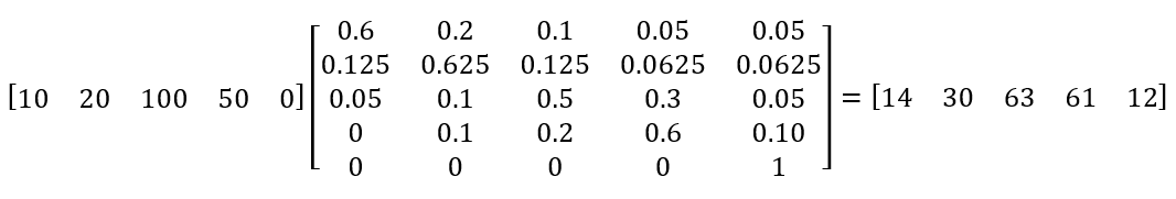
Remember, matrix calculation is done by pairwise multiplying the row elements with the column elements and adding everything up.  In our example, the first result is calculated as 10 times 0.6 + 20 times 0.125 + 100 times 0.05 + 50 times 0 + 0 times 0 which equals 14.  The other numbers are calculated in a similar way.  After one period, this gives us 14 platinum customers, 30 gold customers, 63 silver customers, 61 bronze customers and 12 churners.

We can now continue the analysis and calculate the state after two periods of time.

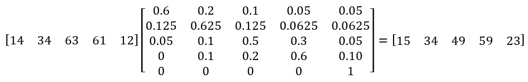
We multiply the previous result with the transition matrix once more.  This gives us 15 platinum customers, 34 gold customers, 49 silver customers, 59 bronze customers and 23 churners.  We can continue the analysis as far as we want.

A Markov reward process is essentially a Markov chain with values which represent rewards assigned to a state or transition.  In a CLV setting, it is obvious that a state reward could represent the customer value in that given state. An example of a transition award could be the cost for upgrading a customer from silver to gold for example.  Note that the reward is negative in this case.  A discounting factor could also be applied to properly discount future rewards to the time of evaluation.  You can see this illustrated here to compute CLV and customer equity.  We start from the value formula as follows:

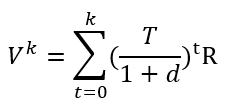
Essentially, V^k is a column vector of expected present values over k periods for each of the states. Let’s work out a small example to illustrate this.  Say we have a 5 by 1 reward vector R which we assume to be constant in time but different for the different states: platinum, gold, silver, bronze and churn.

R = [ 20  10  5  2  0 ]

You can see that platinum customers give a value of 20, gold customers a value of 10, etc. The transition matrix is the same as previously.  We apply a yearly discount factor of 15% and calculate V^k with a time horizon of 3 years.  Doing the simulations according to what we explained earlier results in the 5 by 1 V^k vector you can see illustrated here:

V^k = [ 21 13 6 4 0 ]

The expected present value for the platinum state equals 21, for the gold state 13, etc.

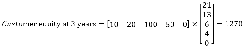
Say we again started with 10 Platinum customers, 20 Gold customers, 100 Silver customers, 50 Bronze customers and 0 Churners as represented by the vector P. We can then calculate the customer equity for the 3 year period using simple matrix multiplication which results into the final customer equity value of 1270.

For more information on Markov Chains (e.g., Markov Decision Processes) for Customer Lifetime Value Modeling, we are happy to refer to our BlueCourses course Customer Lifetime Value Modeling.