RFM Analysis Revisited

Contributed by: Bart Baesens, Seppe vanden Broucke

This article is based on our BlueCourses course Customer Lifetime Value Modeling.

Although RFM analysis is sometimes referred to as a poor man’s approach to CLV analysis, we think it’s a very good way to start doing customer lifetime (CLV) modeling. As always in machine learning, it’s not because it’s simple, that it is necessarily bad. The RFM framework has already been popular since its introduction by Cullinan in 1977.  It’s a well-known and well-developed measurement framework used in marketing across different industries such as banking, insurance, Telco, non-profit, travel, on-line retailers, and even government.  It consists of a set of metrics to monitor customers’ behaviour so as to develop suitable customer relationship management or CRM strategies.  Do note that the RFM framework focusses on existing customers, instead of prospects.

Basically, the RFM famework summarizes the purchasing habits of consumers according to 3 dimensions only.  It essentially builds upon the Pareto principle which states “For many events, roughly 80% of the effects come from 20% of the causes”.  In our case, the events correspond to purchases and the causes to customers.  Or, translated to an RFM setting: 20% of your customers are likely to generate 80% of your profit.  Using the RFM framework, we will try to find out which are those customers who buy or bought recently, frequently and for high monetary values?

Recency measures the time since the most recent purchase transaction.  Frequency measures the total number of purchase transactions in the period examined.  And finally, monetary measures the value of purchases within the period examined.  The combination of these three variables provides a very useful perspective on the value of your current customer portfolio.

Let’s now zoom in on each of the variables of the RFM framework into some more detail.

We start with recency.  As with any RFM variable, it can be operationalized in various ways.  Examples are: how long ago since the customer made a purchase?   This results into a continuous variable.  As an alternative, we can measure it in a binary way as: did the customer make a purchase during the previous day, week, month or year?  Finally, we can also define it in an exponential way.  More specifically, we can define recency as e^(-γt). Here t is the time-interval between two consecutive purchases.  γ is a user-specified parameter which is typically rather small, for example 0.02. Note that by using this procedure, recency is always a number between 0 and 1.  The figure below shows that recency indeed decreases when the time-interval gets bigger.

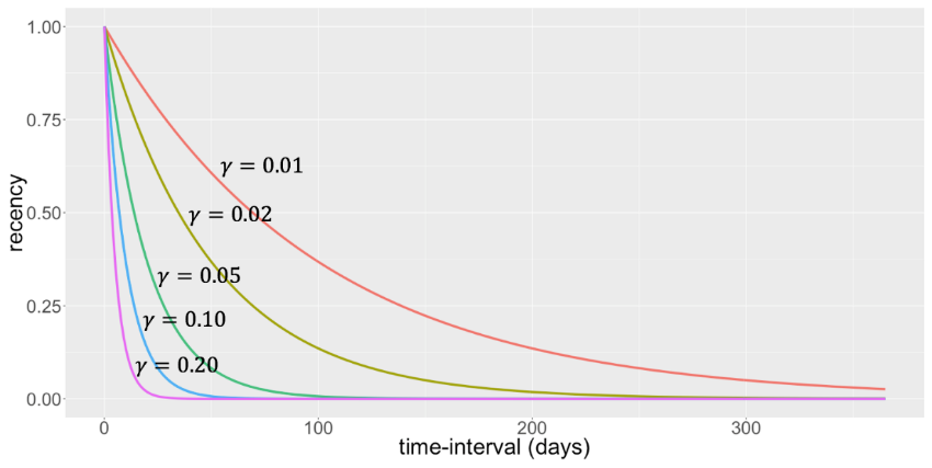
The parameter γ determines how fast the recency decreases. For larger values of γ, recency will decrease quicker with time and vice versa.  But how do you choose γ, you might ask? Well, you could choose γ such that recency has to be equal to 0.01 after 180 days for example. Then γ is -log(0.01)/180.

Frequency is the second variable of the RFM framework.  As said, it measures how frequently the customer buys.  A first way of measuring it is by calculating the average number of purchases per unit of time, such as per month over the last year.  Some frequency calculations will also take the tenure or lifetime of the customer into account and measure it as the total number of purchases divided by the number of months since the first purchase.  According to most research, including the research conducted by myself, the frequency variable is usually the most important of the RFM framework.

Also the monetary variable can be operationalized in various ways.  It can be calculated as the average, maximum or minimum purchase value during the past year.  It can also be measured as the most recent value of a purchase.  Or, we can again take into account the tenure of the customer and consider the total lifetime spending.  Trends can also be looked at.  These features usually turn out to be very predictive in any analytical CLV setting.  Trends summarize the historical evolution of a variable in various ways.  Trends can be computed in an absolute or relative way as follows:

• absolute trend: (M_t – M_(t-x)) / x

• relative trend: (M_t – M_(t-x)) / M_(t-x)

When computing trends, it is important to consider what happens if the denominator becomes 0.  Recent values can also be assigned a higher weighted.  Trends can also be featurized using time series techniques, such as ARIMA or GARCH models.

Interactions between the RFM variables can also be taken into account.  These can be 2-way interactions, 3-way interactions, etc.  Obviously, the thing with interactions is that they usually make a predictive model more difficult to interpret.  Hence, be very careful when considering them.  My practical advice is to only include them when they really add to the predictive performance of your analytical model.  Typically, you will also observe correlations between the R, F and M variables.  A commonly observed correlation is the one between the frequency and monetary variables.  This correlation is not necessarily problematic, but being aware of it is already very important.

We are now ready to start operationalizing the RFM variables such that we can work with them in a meaningful way.  The idea here is to create an RFM score which can then be used for customer segmentation, churn prediction or any other CLV related analytical modeling task.  Obviously, due to continuously changing customer behavior and the external environment, this RFM score should be updated regularly.   Creating an RFM score requires a combination of both analytical skills and business experience.  Let’s elaborate a bit further on this.

Here you can see a very simple example of creating an RFM score.

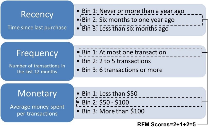
We basically created 3 bins for each of the RFM variables.  The bins are ordinally ordered.  Let’s quickly look at some of them.  For Frequency, bin 1 contains all customers who did at most 1 transaction during the previous month, bin 2 the customers who did 2 to 5 transactions and bin 3 the customers who did 6 or more transactions.  The other variables are binned in a similar way.   Let’s say we have a customer who belongs to bin 2 for recency, to bin 1 for frequency and to bin 2 for monetary.  We can then summarize this into an RFM score of 2 + 1 + 2 or 5.  As said, this procedure can then be used for customer segmentation or to create variables for analytical models.

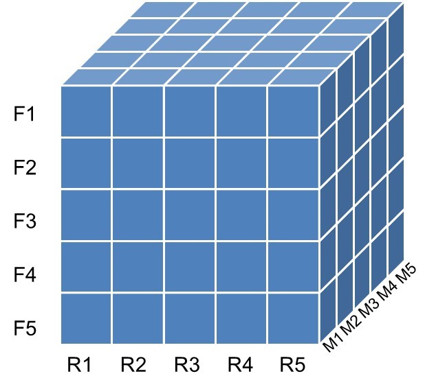
A common way of creating RFM bins is by creating quintiles.  This can be done using either independent or dependent sorting.  Let’s start with independent sorting.  In this case, we sort the data by recency and create 5 quintiles which are labelled as R1, R2 until R5.  The quintile R1 then represents the 20% most ancient buyers.  We then sort by Frequency and also create 5 quintiles.  F1 represents the customers that buy least frequently.   Finally, we do the same for the monetary variable, sort and create 5 quintiles: M1 until M5 with M1 representing the lowest average spenders.  The final RFM score can then be used as a cluster indicator or even as a predictor for an analytical model.  Note that the best customers are typically assumed to be in quintile 5 for each RFM variable or cluster 555.  These represent the customers that have purchased most recently, most frequently and have spent the most money.

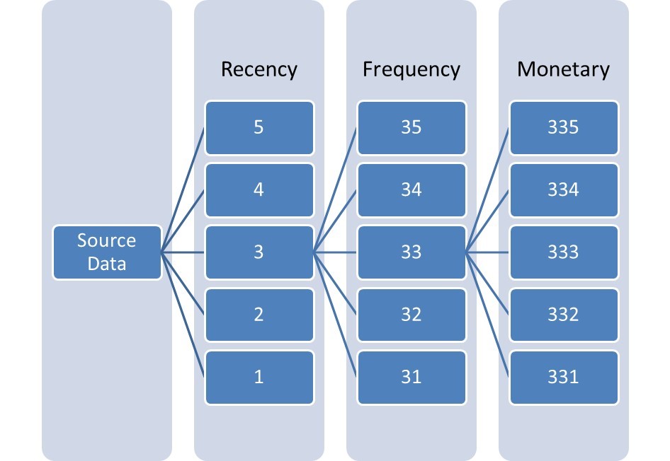
Dependent sorting works in a strict sequential way.  It starts with the Recency variable first and creates the 5 quintiles.  Each Recency quintile is then further binned into 5 Frequency quintiles.  Each resulting RF bin is then further binned into 5 quintiles based  on the Monetary variable.  As with independent sorting, the final RFM score can be used as a cluster indicator or variable in a predictive analytical CLV model.  Note that scientifically, to the best of my knowledge, it is not possible to state which one is best: independent or dependent sorting.

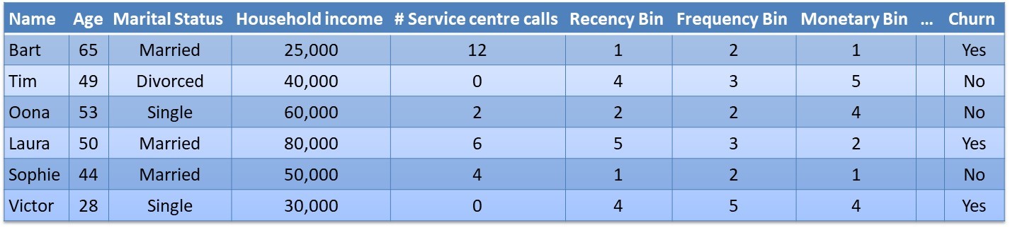
The RFM variables can be used as input variables for various analytical CLV models such as churn prediction, response modeling, customer segmentation and obviously also CLV analytical models.  The bottom table illustrates a churn prediction data set which combines the RFM variables with other customer specific information such as age, marital status, etc.

Let’s now zoom out of the original marketing context and do some out of the box thinking.  Essentially, recency quantifies the recency of an event, frequency the frequency of events and monetary the impact, intensity or reach of an event.  Defining the RFM variables in this more general way, opens up perspectives for their use in other settings.  The RFM variables are commonly used in fraud analytics.  Think about credit card fraud as an example.  Here, R can refer to the recency of a transaction, F to the frequency and M to the monetary value.  In web analytics, the recency can represent the recency of a web site visit, the frequency the frequency thereof and the monetary variable can represent the duration of the visit.  In a social media setting, we can look at the recency of a post, the frequency of posts and community size that is reached with the post, such as followers, retweets, shares, etc.

Let’s conclude the discussion of the RFM framework with some closing thoughts.  A key advantage of the RFM framework is that it is simple and easy to understand and calculate.  It provides a compact and powerful representation of customer behavior.  We consider it to be an ideal approach to build your first CLV models.  Remember, when doing analytics it is always wise to start off simple and then gradually sophisticate your models.