
This article first appeared in Data Science Briefings, the DataMiningApps newsletter. Subscribe now for free if you want to be the first to receive our feature articles, or follow us @DataMiningApps. Do you also wish to contribute to Data Science Briefings? Shoot us an e-mail over at briefings@dataminingapps.com and let’s get in touch!
Contributed by: Bart Baesens
A social network is a network of nodes connected with links. Think of customers calling each other, people exchanging emails, companies lending money to each other or fraudsters collaborating as part of a collusion.
The nodes in social networks are usually not randomly linked together. Since these networks typically represent people’s social interactions, there is always a reason for the connection. The reason for links to specific people is that they share a common property. For example, common interests or same origin. Homophily is a concept that stems from sociology where it usually described as “people have a strong tendency to associate with others whom they perceive as being similar to themselves in some way, e.g., live in same city, have same hobbies or interest”. It is also often referred to as “Birds of a feather flock together”. The figure shows an illustration of homophily in a call network.
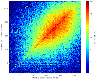
Fixman, Martin et al. (2016) illustrated that people tend to call other people of the same economic status. You can see a clear correlation between the monthly caller and monthly callee income. Hence, this is strong evidence of homophily between people with similar income levels.
Homophily can also occur in fraud networks if fraudsters are more likely to be connected to other fraudsters, and legitimate people are more likely to be connected to other legitimate people. Homophily depends on the connectedness between nodes with the same label and the connectedness between nodes with the opposite label. We elaborate on this in what follows.
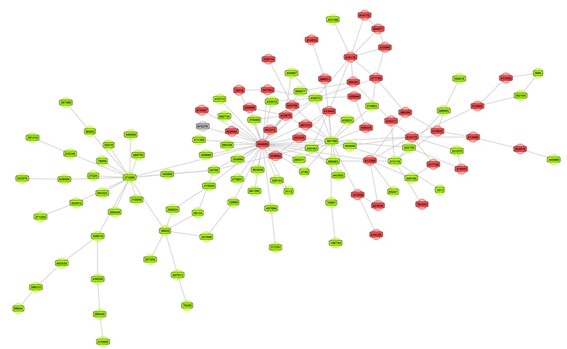
Sometimes a visual inspection of a network can already signal clear signs of homophily. Look at the below network where the green nodes represent legitimate customers and the red nodes fraudsters. The visual inspection clearly reveals signs of homophily.
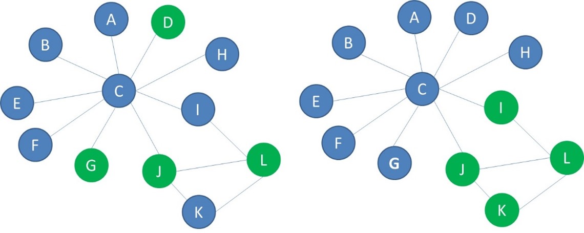
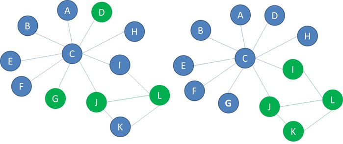
Below you see another example of two networks with blue and green nodes. In the network on the left, the green nodes are randomly spread through the network. This network is not homophilic. The green nodes in the network on the right are connected to each other to a larger extent. This network is homophilic.
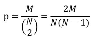
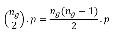
Before defining homophily we need to define the connectance of a network, which is the probability that 2 nodes are connected. Say we have a network with N nodes and M edges. The connectance is then the ratio between the actual number of edges and the number of edges if the network was fully connected, the latter being the number of combinations of 2 out of N:
In the below example, the connectance equals 20%.

Dyadicity measures the connectedness between nodes with the same label. As an example let’s look at the below two networks. Both of them have 12 nodes, 8 that are blue and 4 that are green. Clearly the distribution of the green and blue nodes is different. In the network on the left there is only 1 edge between the green nodes, but on the right there are 4. There is higher connectedness between green nodes in the network to the right.
Dyadicity measures the number of same label edges compared to what is expected in a random configuration of the network, in other words, if the labels were randomly distributed. Say ng represents the number of green nodes. The expected number of green label edges then becomes: the number of combinations of 2 out of ng times p, which, as you recall, is the probability of two nodes being connected.
In the below example, there are 8 blue nodes, 4 green nodes and the connectance is 0.2, so the expected number of edges connecting green nodes is 4*3/2*0,2=1,2. Finally, you compute the dyadicity or D by dividing the actual number of same label edges with the expected number of same label edges. In our below example, the dyadicity becomes 3,33.

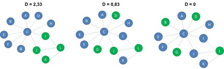
If the dyadicity is greater than 1 we say that the network is dyadic because nodes with the same label are more connected amongst themselves. This is the case for the network to the left. If the dyadicity is almost equal to one, the distribution of the labels is the same as in a random network. You can see an example of this in the middle network. If the dyadicity is less than 1 we say that the network is anti-dyadic since nodes with the same label are less connected amongst themselves. You can see an example of this in the network to the right.
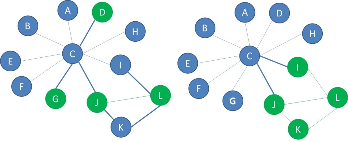
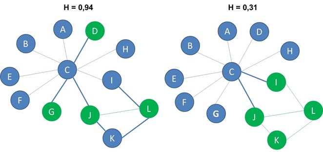
For a network to show signs of homophily, it is not enough for nodes of the same label to be more connected. There should also be fewer connections between nodes of opposite labels. This is measured with heterophilicity, which is the other parameter you need to capture the interplay between the network structure and node properties. Heterophilicity measures the connectedness between nodes with opposite labels and thus how much interaction there is between the nodes with different labels. Let’s take a look at the below two networks, which both have 8 blue nodes and 4 green nodes. We represented the cross-label edges with a thicker line. In the network on the left there are 6 cross-label edges. In the network on the right, there are 2 cross-label edges.
Heterophilicity measures the connectedness between nodes with different labels compared to what is expected in a random configuration of the network. The expected number of cross label edges, that is edges that connect a blue node and a green node, equals nb*ng*p . We multiply the number of each type of node, denoted here with nb and ng with the network connectance, p. In the network with 8 blue nodes, 4 green nodes and connectance equal to 0.2, the expected number of cross label edges is 8 times 4 times 0.2 or 6.4 which we could round to 6. Finally, we compute heterophilicity by dividing the actual number of cross label edges with the expected number of cross label edges which gives us 0,31.
Below you can see the two networks from before. The network on the left has heterophilicty of 0.94 and the network on the right has heterophilicity of 0.31.
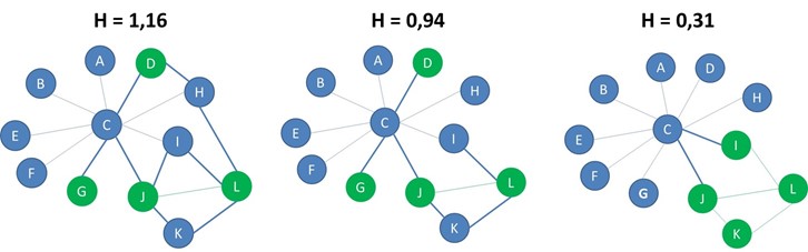
If the heterophilicity is greater than 1 we say that the network is heterophilic because there are more connections between nodes of different labels. If the heterophilicity is almost equal to one, the distribution of the labels is the same as in a random network. If the heterophilicity is less than 1 we say that the network is heterophobic since nodes of opposite labels do not tend to be connected. Note that we added some extra cross-label edges in the network to the left, which results in a heterophilicity of 1,16 which implies the network can be labelled as heterophilic. In terms of heterophilicity, the network in the middle is random, whereas the network to the right is heterophobic.
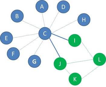
We now learned how to compute the dyadicity and heterophilicity of a network. Both parameters are necessary to capture the detailed interplay between the network structure and node properties. But how do they relate to homophily? One of the essential questions before doing predictive analytics using networked data, is deciding whether the predictive models might benefit from social network analytics. In the case of predicting fraud, do the relationships between people play an important role, and is fraud a contagious effect in the network? Are the two labels randomly spread over the network, or are there observable effects indicating that there is a social phenomenon, in other words, do fraudsters tend to cluster together. In terms of the network structure, this means that connections amongst nodes with the same label are more common, in other words that the network is dyadic, and that connections between nodes with different labels are rarer, in other words., that the network is heterophobic. As you recall, homophily is characterized by nodes of the same label being more connected to each other and nodes of opposite labels being less connected to each other. The network shown below has dyadicity greater than 1 and heterophilicity less than 1. Therefore, we can infer that this network is homophilic and use it for predictive analysis.
Now you should be able to determine whether a network is homophilic based on its dyadicity and heterophilicity. Note however, that these are not absolute values. The network can be homophilic even though it is only either dyadic or heterophobic, or if the values for dyadicity and heterophilicity are only slightly different from one. The important thing is that the distribution of the labels is not random and we can use the information to make predictions in the network. A network that exhibits evidence of homophily, is worthwhile to investigate more thoroughly. For each node, we will do featurization, which means we extract features that characterize the node based on its position in the network. The predictive analytics technique used subsequently (e.g., logistic regression, decision trees, XGBoost, neural networks, …) can then indicate whether these features turn out to be significant or not.
Fixman, Martin, et al. “A Bayesian approach to income inference in a communication network.” Advances in Social Networks Analysis and Mining (ASONAM), 2016 IEEE/ACM International Conference on. IEEE, 2016.