
Contributed by: Bart Baesens
This article first appeared in Data Science Briefings, the DataMiningApps newsletter. Subscribe now for free if you want to be the first to receive our feature articles, or follow us @DataMiningApps. Do you also wish to contribute to Data Science Briefings? Shoot us an e-mail over at briefings@dataminingapps.com and let’s get in touch!
This article is about Bayesian networks which we believe is too much ignored in today’s analytics jungle blitzed with technological buzzwords such as deep learning, reinforcement learning, etc. Let’s revisit Bayesian networks, one of the technologies we personally think have been too much overlooked and have great potential in many applications.
A Bayesian network represents a joint probability distribution over a set of categorical, stochastic variables (continuous extensions have been developed, but let’s keep it simple at the moment). It consists of two parts. A qualitative part specifies the conditional dependencies between the variables represented as a graph, and a quantitative part specifies the conditional probabilities of the variables. Here you can see an example of a Bayesian network:
Given its attractive and easy-to-understand visual representation, a Bayesian network is commonly referred to as a probabilistic white box model. More formally, a Bayesian network consists of a graph G, which is a directed acyclic graph that consists of nodes and arcs depicting dependencies, and θ representing the conditional probability distributions. Bayesian networks allow to combine both domain knowledge with patterns learned from data. Hence, they could be interesting alternatives to model settings in which not a lot of data is available yet. Small data, can you believe it? Even a bigger challenge than big data if you ask me. Small data can occur in settings with new products or very specific products such as a project finance credit portfolio, or even very rarely occurring diseases with not a lot of patient data.
θ contains a parameter θxj|π (xj), which is the probability of observing a value for xj given the values of the direct parent variables of xj in G, represented by π(xj). The Bayesian network then represents the following joint probability distribution for n variables x1, …, xn:
![]()
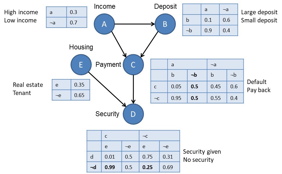
Let’s now reconsider the above Bayesian network and illustrate how we can reason with it. It has the following five variables, which are represented as nodes: Income, Deposit, Payment, Security, and Housing. Each variable has been categorized into two states. For example, Income has been categorized into High Income and Low Income. The arcs depict the dependencies. For example, Deposit is conditionally dependent on Income. Payment is conditionally dependent on Income and Deposit. Income is not conditionally dependent on any other variable that is included. The tables represent the θ parameters, or in other words, the conditional probabilities. For example, the probability of observing High Income equals 0.3, and the probability of observing Low Income equals 0.7. The probability of observing Large Deposit given High Income equals 0.9, and the probability of observing Small Deposit given High Income equals 0.1. What do you think the probability of default is, given Low Income and Small Deposit? Well, if you look it up in the table, you will see that the probability of default, given Low Income and Small Deposit equals 0.8. You can now use this network and its probability tables to calculate various probabilities of interest. In fact, you can use the network as a classifier. Consider a customer applying for a loan. The customer has a high income (a), a small deposit (¬b), no security (¬d), and owns real estate property (e). What is the probability that a customer with these characteristics will default or pay back the loan? Well, let’s calculate the joint probability of a, ¬b, c, ¬d, and e according to the network. As explained earlier, this joint probability factors according to the dependencies observed in the network, or in other words,
P(a, ¬b, c, ¬d, e) = P(a)*P(¬b | a)*P(c | a, ¬b)*P(¬d | c, e)*P(e).
Direct table lookup then yields the following:
P(a, ¬b, c, ¬d, e) = 0.3*0.1*0.6*0.99*0.35 = 0.006237.
Similarly,
P(¬c, a, ¬b, ¬d, e) = P(a)*P(¬b | a)*P(¬c | a, ¬b)*P(¬d | ¬c, e)*P(e).
Again, direct table lookup yields the following:
P(¬c, a, ¬b, ¬d, e) = 0.3*0.1*0.4*0.25*0.35 = 0.00105.
We can now apply Bayes theorem to calculate the conditional probabilities as follows: P(c | a, ¬b, ¬d, e) = 0.006237/(0.006237+0.00105) = 0.855908. Similarly, P(¬c | a, ¬b, ¬d, e) = 0.144092. Hence, according to the winner-takes-all rule, the customer should be assigned class c or thus default.
Learning a Bayesian network is essentially a two-step process. In Step 1, you learn about the structure of the graph G. In Step 2, you learn the θ parameters. Notice that these usually correspond to the empirical frequencies as observed in the data.
The most difficult part in building a Bayesian network is learning the network structure. Two methods can be followed here: the domain expert method and the data-driven method. In the domain expert method, the structure of the network is learned by interviewing domain or business experts. This method will be especially relevant in domains with large amounts of business knowledge. Consider the example of a low default portfolio. To build the Bayesian network, you can start by interviewing various credit experts dealing with the low default portfolio. This is Step 1. In Step 2, you list all the important variables based on the interviews. In our example, there might be variables such as liquidity, solvency, profitability, and so on. In Step 3, the dependencies between the variables are drawn based on the input from the credit experts. In this case, an arrow can be drawn between solvency and default risk, for example. Obviously, conflicts might arise between the knowledge and experience of the credit experts. These disagreements will need to be solved in Step 4. After the network structure has been set up, the probabilities can be estimated from the data in a final step. The network is now ready for use and inference. The Bayesian network structure can also be learned in a data-driven way. This will be appropriate in settings where no domain or business knowledge is available. Various methods have been developed to learn Bayesian networks from data. They are all quite complex and we refer to the literature for more information on this. Most of these methods rely on analyzing dependencies or correlations between variables. Based on calculating these correlations, the dependencies between the various variables are determined. It is very important to note here that these dependencies are not to be interpreted in a causal way. Remember the distinction between correlation and causation. Various empirical studies have shown that building Bayesian networks from data is not an easy exercise. A final method is a hybrid method that combines both the domain expert and the data-driven method.
To summarize, we discussed Bayesian networks as probabilistic white box models. It is our firm believe that they have great potential for analytical modeling.