
Contributed by: Bart Baesens, Seppe vanden Broucke
This article first appeared in Data Science Briefings, the DataMiningApps newsletter. Subscribe now for free if you want to be the first to receive our feature articles, or follow us @DataMiningApps. Do you also wish to contribute to Data Science Briefings? Shoot us an e-mail over at briefings@dataminingapps.com and let’s get in touch!
In this article, we take a closer look at LIME. LIME is a way to make machine learning models more interpretable and stands for Local interpretable model-agnostic explanations and was developed by Ribeiro et al in the KDD paper:
Ribeiro, Marco Tulio, Sameer Singh, and Carlos Guestrin. “Why should I trust you?: Explaining the predictions of any classifier.”, Proceedings of the 22nd ACM SIGKDD International Conference on Knowledge Discovery and Data Mining, ACM 2016.
Essentially, LIME implements a “local surrogate” model to provide predictions. More specifically, LIME helps to explain single individual predictions, not the data as a whole, a particular feature (like partial dependence plots) or the model as a whole. It works on any type of black box model, neural networks, SVMss, XGBoost, etc. It is model-agnostic and works with tabular and other types of data (e.g. text, images).
Assume we have trained a black box classifier b and want to explain a given instance Assume that the prediction of the black box classifier equals b(x_i) = p(y=1|x_i)=0.78 for the case of binary classification and we want to know why? The main idea of LIME is as follows.
- First, create a new dataset containing permutated samples around x_i and have the black box model provide predictions for these.
- In a second step, train a local, interpretable model on this data set and use it to offer explanations. This model is weighted by taking a sample based on the proximity of the permuted instances around x_i. LASSO regression or a regression tree are commonly used for this purpose.
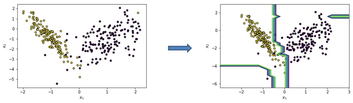
Example data set to illustrate LIME
You can see this illustrated in the figure above. Assume we start from a binary classification data set with 2 features: x_1 and x_2. We then train a random forest classifier which results in the decision boundary illustrated in the figure to the right.
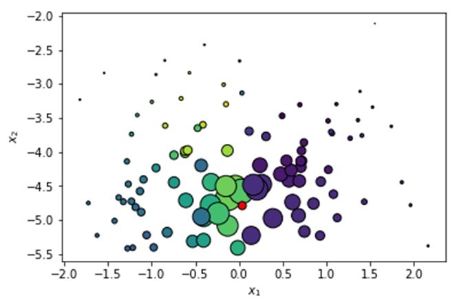
We now select an instance we wish to explain. Let’s say we would like to explain the red observation in the figure below.
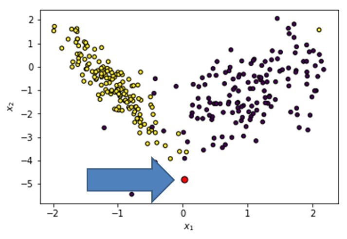
Instance to explain in LIME
We first create a permuted data set which we obtain by uniform sampling for tabular data. The observations sampled around the red instance under study are all weighted: the further from the instance the lower the weight as you can see from the smaller size of the blue dots. Note that most LIME implementations use an exponential smoothing kernel to do this, which is similar to t-SNE:
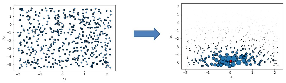
Permuted data set in LIME
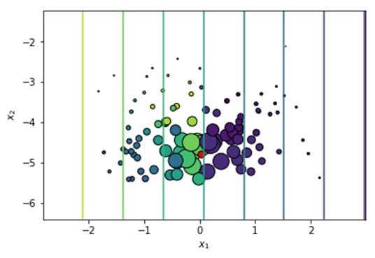
We can have the black box model, which is a random forest in our case, make its predictions or thus calculate its probabilities as shown in the figure below:
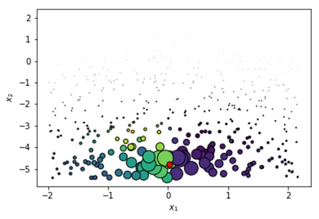
Black blox predictions in LIME
Finally, we sample from the perturbed data set based on the weights — higher weights have a higher chance to be sampled:
Sampling from perturbed data set in LIME
A simple machine learning model is then trained on this perturbed data set. Very often, LASSO regression is used, as this model will serve as a sparse explainer for the instance under observation. Note that the output of this regression model is now a continuous value representing the predicted probabilities of the black box model. This provides us with a simple, local decision boundary which can be easily inspected, e.g. by inspecting the coefficients of the model or deriving the smallest amount of changes that would need to happen to the instance for its probability to switch from <= 0.50 to > 0.50:
 Output of regression model in LIME
From our figure, it is clear to see that variable x2 is not important. The line going through x1 equals 0 is the most important since the class on the right side of it is the other class:
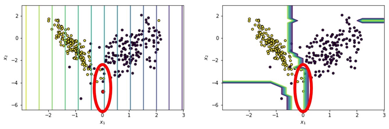 Decision boundaries in LIME
You can nicely see that the decision boundary of the “explanatory model” approximates the decision boundary of the black box or random forest model around the instance under study.
LIME can also be applied to non-tabular data such as text or images. Using non-tabular data changes how the perturbation is performed. In case of text data, new texts are created by randomly removing words from the original text. E.g. if the dataset is represented with binary features for each word (bag of words), this can be done in a very straightforward way. For images, perturbing individual pixels does not make a lot of sense. Instead, groups of pixels in the image are perturbed at once by “blanking” them (removing them from the image). These groups are called “superpixels”, based on interconnected pixels with similar coloring. They can be found using for example a k-means clustering.
You can see this illustrated in the figure below from the original paper by Ribeiro et al. This figure show the superpixels explanations for the top 3 predicted classes, with the rest of the image grayed out. The top 3 classes predicted are electric Guitar, acoustic guitar and Labrador.
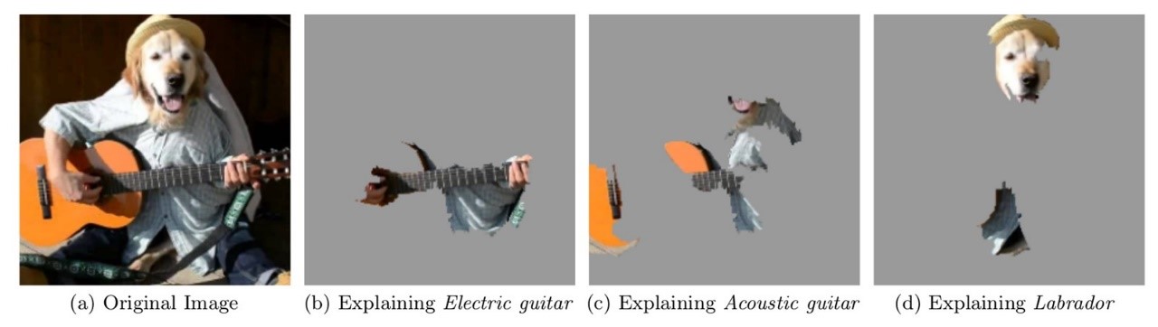
LIME on non-tabular data (source: Ribeiro et al.)
Defining a neighborhood around an instance to define the weights is difficult. For example, the distance measure or bandwidth of the exponential smoothing kernel used by LIME can heavily impact results. As a simple alternative, one can also select the k nearest neighbors around the instance under study, but do note that we then still need to decide upon an appropriate k. Choosing the simple model is also somewhat arbitrary. For example, the tuning of the regularization parameter of the LASSO regression can impact the results. The main advantage is that LIME is easy to understand and works on tabular data, text and images.
Here you can see some references to LIME implementations in R and Python:
- Python (lime): https://github.com/marcotcr/lime
- R (lime): https://lime.data-imaginist.com/
- Python (eli5): https://eli5.readthedocs.io/en/0.1.1/lime.html
- R (iml): https://cran.r-project.org/web/packages/iml/index.html