How Incorrectly Specified Targets Harm Predictive Models

Contributed by: Seppe vanden Broucke and Bart Baesens. This article was adopted from our Managing Model Risk book. Check out managingmodelriskbook.com to learn more.

Many analytical tasks require a label or target to be specified. This target will then be used to steer the building of the analytical model (e.g. a regression model, decision tree, neural network, etc.). It is quite obvious that if the target is incorrectly specified or defined the analytical model will learn the wrong things.

Goodhart’s Law states that “when a measure becomes a target, it ceases to be a good measure.” At their core, what most machine learning models do is to optimize a metric: given a certain list of targets, find a model which results in the lowest error or loss towards predicting those targets.

Hence, it is important that this target is appropriately specified in close collaboration with the business end users in order to fully understand what it measures. More so, any risk that might be present related to the optimization of metrics has a danger of being exacerbated when used in a predictive modeling setup.

Let’s illustrate this with a couple of examples. A first example concerns Customer Lifetime Value (CLV) modeling. Here, the CLV target is usually defined as follows:

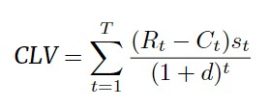
The key elements are:

• The costs at time t: Ct
• The revenue at time t: Rt
• The probability the customer is still alive at time t: st
• The discount rate: d
• The time horizon: T

Let’s elaborate on each of these parameters into some more detail. First the time horizon. Theoretically, this should be infinity. Unfortunately, this is practically infeasible since it’s simply impossible to predict that far in the future. Based on our business experience, we would suggest to set it to three or five years at maximum. Next, we have the discount rate. Theoretically, we don’t know this one yet as we would have to wait until T to observe it. A difference also needs to be made between the monthly versus yearly discount rate (one plus the yearly discount rate equals one plus the monthly discount rate raised to the power twelve). It is typically chosen according to the company’s policy. One option here is to use the Weighted Average Cost of Capital or WACC. In case the short-term relationship is considered important, a high discount rate is chosen, such as 15% annually. In case a long-term relationship is considered important, a low discount rate is chosen, such as 5% annually. A higher discount rate typically implies a lower CLV since future cash flows are worth less now. Hence, it is recommended to be conservative when setting the discount factor. The revenue and costs should incorporate both direct and indirect revenues and costs if possible. Furthermore, they should include numbers from the various departments such as sales, marketing, IT, etc. Both Rt and Ct can be estimated themselves and as such be the result of different analytical models. Finally, we have the survival probability st. Remember, this represents the probability the customer is still alive at time t. It is typically estimated using bespoke survival analysis models.

With so much uncertainty, assumptions and models being used, even, to provide targets to be used by other models, it is clear that any incorrect setting of the targets can lead to an incorrect model down the line. Parameters (such as the discount rate or costs) might also change as time progresses, so models are immediately outdated the moment they’re trained. In fact, most of the targets we end up defining to provide to a model end up being proxies for what it is we actually want to know or optimize.

Let’s look at a different example. In fraud detection, it might sound desirable to label our instances (claims, transactions, etc.) as fraudulent based on formally confirmed historical occurrences of fraud. Sadly, since such a formal closure and confirmation of fraud can take a long time in many settings, this leads to the issue of not having enough positive cases to train on, so that the decision is often made in this setting to consider suspicious cases as positive instead. Perhaps some of these will not result in a formal confirmation, but at least such a model could already be useful. Typically, a suspicious case will lead to additional efforts and costs being spent in order to e.g. collect evidence, gather documentation, bring it forward to a court case, etc., so that having a model which can output a shortlist would already be beneficial. Still, we have already changed our target definition. Now let’s say we continue to train our model as such and try it out. Assume that we get the (unrealistically good) results of this model having a 90% recall score and 100% precision. In other words: it captures nine out of ten fraudulent cases in the test set, and does not predict any cases as fraudulent which turn out not be. Sure, this sounds like a fantastic result, but again we can show that this is in fact not necessarily the case. More specifically, let us consider the fact that all of these cases come with a certain amount of value which can be recovered. This can be some paid out amount by the firm which we get back, together with any additional sanctions the fraudster needs to pay. We also need to spend some amount of time and money as mentioned before to work on the case, which should also be taken into account. Now let’s say that our model is detecting the 90% suspicious cases with the lowest recovery value, and misses the 10% most valuable ones. In this case, we actually might even end up losing money for those cases where the amount to be gained is less than the costs it would take to work on it.

Now what we could do here, obviously, is to apply a post-hoc filtering on our model’s predictions and only retain the top-n cases for which we know the associated value is high enough. Although this is a relatively common practice, it sadly fails to inform the model during training of the notion that it should try to focus more on high-value cases than low value ones. What we could do is to change our target definition once again and have our model predict the amount that can be recovered, and setting it to zero for the non-suspicious cases. We now have a regression problem rather than a binary classification one. We could also stick to binary targets, but only consider as positives those cases where there was not only a suspicion of fraud but where the associated value was also high enough.

To make the above even more cumbersome to deal with, it is in many settings not even possible to determine the amount that could be recovered if a case is fraudulent (and proven as such) when we are still early in the underlying business process. As such, even this value might be something that needs to be estimated. In fact, we have constructed modeling pipelines where first, a model is used to estimate the true value of a case based on the features available at case entry, which is then used as an additional feature by another model that predicts whether a case is suspicious and is trained to optimize the recovered amount. This is already a lot more complicated than just working with a list of binary labels. In addition, we have seen outcomes from such a setup where the model either believes it to be most optimal to regard none of the cases as suspicious or to just base its top-n on the predicted (or true) case recovery value, disregarding all other features. The former shows that the costs involved in checking cases are specified as being too high. The latter shows that the model believes you’re best off by checking the n most valuable cases. Disregard the other signals: if only one of those cases turns out to be fraudulent, you’ve gained your money back! Again, the outcome here will change based on how you tune costs, n, and what you consider as “value” of a case.

The above might sound extreme or far-fetched, but it does happen a lot in practice and can make the difference between an underwhelming model and a powerful one. Not just for fraud, but many other settings as well. Let’s turn our attention to credit scoring where one wants to distinguish bad payers from good payers. But again, what actually is a bad payer? Let’s assume we label a customer who has been one month in payment arrears as a bad payer. Upon closer consideration, these could actually turn out to be very profitable customers in case they successfully pay back all their arrears penalties. This obviously could reverse the problem: one particular group of interesting profitable customers are the ones who have been one month in payment arrears and pay everything back and the “negative” ones are the complementary ones. Again not as easy as it appears on first sight.

The same happens in churn prediction as well. Again, do we just care about any customer leaving, or rather about those where we would have expected a high CLV (again perhaps as predicted by another model) or which were buying a lot in the past? Another way how label definitions typically end up being incorrect is by not carefully considering the different time frames involved concerning at which moment the features are extracted versus at which moment the outcome of the target is realized. The CLV example above already illustrated this through the time horizon T. Typically, for predictive models, the target will be something that will occur or be realized somewhere in the future, which you want to predict based on a snapshot of what you observe today. Sometimes, however, we see practitioners doing the following:

The figure above shows three customer instances. A snapshot of all the customers’ features is taken based on a specific vantage point. Very often, this is based on the actual, current state as is stored in e.g. an operational data base, hence, “today”. The target then is based by inspecting the history of each customer. Customer A is still with us at the present moment so they would get a negative label. B and C have churned so they get a positive label. This modeling approach is, however, completely inappropriate. What we are doing here is predicting something that happened in the past based on what we observe afterwards, which isn’t very hard. Some people will try to defend this approach by claiming that they would then look at the highest-scored false positives of the model and interpret those cases as instances which look like they should have churned already, but didn’t. Again, this is ill-advised. Not only did you provide your model with badly specified targets, but what would you do in case the model would act as a perfect oracle (which would not even be too surprising since we’re predicting the past here) and hence wouldn’t have any false positives.

Of course, the approach we should instead use looks as follows:

The difference here is that we now use a point in the past to construct our feature snapshot from, and then look forward into the future over some observation period to see which customers have churned and which ones did not (or not yet). Note that the length of the observation period will have a direct impact on how many positive labels you will extract (in the figure above, customers B and C have churned during the observation period but A did not). Secondly, we could also decide to first have a period of “missed opportunities”: instances which churn but are considered to be such soon-in-the-future churners that it is not worthwhile to detect them. Since these will typically also be the easier cases to spot by the model, we might even decide to drop such cases from the train set altogether and adjust the data perimeter.

Again, combined with what was discussed above, here too, one can think of many different possible ways to construct the target. Even the type of churn could play a role. For example, consider a churn model used at a bank. It is doing a good job, though further investigation reveals that the model mainly detects churners which just had a conversation with their financial advisor related to the possibility of getting a mortgage to purchase their first house and weren’t able to get an offer (or one they liked). Since people talk with different banks when applying for a mortgage (and are prepared to switch banks), it’s only natural that this results in a high amount of churn. Note that this can happen even when there aren’t any features in the original data set pertaining to “failed talks related to a mortgage”, as the model can learn it through other correlations (such as age, marital status, recent change in occupation, investment or saving behavior, etc.). The model itself isn’t wrongly constructed, but the target definition requires redefining: we’re interested in churning customers, but not due to the reason of a rejected mortgage application, as such cases are typically impossible to turn around anyway and the bank is likely not in a position to change its mortgage terms and conditions.

Constructing a solid target definition for churn for financial institutions is generally very hard. What is a churner, anyway? Someone who cancels all their checking, savings, and investment accounts? People will rarely do so and typically leave one account open (a so called sleeping account with only a couple of euros on it or so). So perhaps it is someone who hasn’t executed any transactions for more than a year? Two years? But you will always find exceptions to this rule, and these are typically customers you don’t want to disturb or anger.

Hopefully, the point is clear by now. The main problem here is that true business objectives are often composed out of hard to measure and multiple parts (the objectives are indeed often very subjective), on top of which it is hard to find a clear weighting between them. Multi-objective optimization is a hard research topic in general, and machine learning techniques also have a hard time dealing with these settings. They typically want the analyst to specify one single target and/or one single loss function which can be optimized.

Let’s take a look at another interesting example, taken from the paper Does Machine Learning Automate Moral Hazard and Error (2017). Here, the researchers investigate which features in a patient’s medical record are most predictive of a (future) stroke. It turns out that many of the most predictive factors (like having had an accidental injury or a colonoscopy) actually don’t make sense as risk factors for stroke. Upon closer inspection, it turned out that the labels they were given were the result of a somewhat biased measuring process. To quote from the paper: “Our measures are several layers removed from the biological signature of blood flow restriction to brain cells. Instead we see the presence of a billing code or a note recorded by a doctor. Moreover, unless the stroke is discovered during the ED visit, the patient must have either decided to return, or mentioned new symptoms to her doctors during hospital admission that provoked new testing. In other words, measured stroke is (at least) the compound of: having stroke-like symptoms, deciding to seek medical care, and being tested and diagnosed by a doctor.”

However, many other factors influence this overall process other than those related to biological risk factors to get a stroke: e.g. who has health insurance or can afford their co-pay, who can take time off of work or find childcare, cultural factors, sociodemographic background and more. As a result, the model was largely focusing on people who were utilizing healthcare a lot (and got a stroke) rather than answering the general question on who is at risk to get a stroke.

This problem shows up all over the place, and can even become exacerbated when AI or machine learning is used, especially when prescriptive actions are undertaken based on a model or recommendations are made by it. For instance, a key metric of interest in the area of web analytics is the bounce rate. This used to be defined as the percentage of site visits where the visitor left instantly after having seen one page. Although this is still commonly used, many organizations and content providers have found that this metric is a rather weak proxy for what we really want to measure: engagement. That is, perhaps it doesn’t matter that someone only clicked on one of our articles, if they stayed a long time on the page. As such, a more meaningful definition is to consider the time the visitor spent on your website. If this is less than, say ten seconds, it clearly shows that the visitor was not engaged at all with your web site content and could thus be considered as a bounce. What would happen if we start to adjust our content based on the predictions on some model which tries to tell what we can expect in terms of bounce rate (or time spent on page). Perhaps journalists of news sites will be pushed into a setting where they will start writing more verbose, long-form content? What happens if we use number of visits instead? Most likely this will lead to clickbaity titles being used. Google has utilized the number of hours someone spends watching YouTube as a proxy for how happy users were with the content. Sadly, engineers also found out that this had the unwanted side effect of incentivizing conspiracy theory videos, since convincing users that the mainstream media is lying typically keeps them watching more YouTube, even if it is just to have a laugh.

The problem is that most metrics we end up using tend to focus on short-term gains, but fail to capture long-term, strategic, societal aspects, as other scholars have also argued, e.g. in the paper The problem with metrics is a fundamental problem for AI (2020). All of this goes to say that we should be very careful in the way we set our targets or labels. These positives and negatives might look very inconspicuous, but the contrary is often the case: they contain a lot of hidden assumptions and shortcuts.