QA: What is the best way to deal with skewed data sets which are common in e.g. fraud detection or churn prediction?

By: Bart Baesens, Seppe vanden Broucke | Read and comment on this article on Medium

This QA first appeared in Data Science Briefings, the DataMiningApps newsletter as a “Free Tweet Consulting Experience” — where we answer a data science or analytics question of 140 characters maximum. Also want to submit your question? Just Tweet us @DataMiningApps. Want to remain anonymous? Then send us a direct message and we’ll keep all your details private. Subscribe now for free if you want to be the first to receive our articles and stay up to data on data science news, or follow us @DataMiningApps.

You asked: What is the best way to deal with skewed data sets which are common in e.g. fraud detection or churn prediction?

Our answer:

Good question indeed! Various procedures can be adopted to deal with skewed data sets that have e.g. less than 1% of the minority class. Common procedures are undersampling the majority class and oversampling the minority class. Personally, we have a preference for undersampling the majority class since oversampling creates correlations between the observations. In addition, you’ll end up with a smaller data set which fits nicer in memory and reduces training time.

In the industry, we often witness a 80/20 distribution to develop classification models although the optimal ratio may depend upon the data set characteristics. In our research, we recently experimented with the Synthetic Minority Oversampling Technique aka SMOTE, developed by Chawla, and obtained some good performances with it. The idea here is to create random synthetic examples of the minority class observations by combining them. State-of-art techniques improve upon this idea, e.g. by sampling minority instances in a more carefully guided manner, preventing possible overlap between the generated instances and the majority class instances (Safe-SMOTE). Very important to be aware of is that if you adopt any of these techniques the posterior class probabilities are biased. This is okay if you are only interested in ranking, but if you require well-calibrated probabilities (e.g. as in credit risk modeling) a re-calibra tion is needed. One straightforward way to do this is by using the following formula (Saerens, Latinne et al., 2002):

,

whereby Ci represents class i (e.g. class 1 for the minority class and 2 for the majority class), p(Ci) the prior probability (e.g. p(C1)=1% and p(C2)=99%), pr(Ci) the resampled prior probability due to oversampling, undersampling or other resampling procedures (e.g.pr(C1)=20% and pr(C2)=80%), and pr(Ci|x) represents the posterior probability for observation x as calculated by the analytical technique using the resampled data. Note that the formula can be easily extended to more than 2 classes. The below table shows an example of adjusting the posterior probability in a fraud detection context, whereby p(C1)=1%; p(C2)=99%, pr(C1)=20%; and pr(C2)=80%. It can be easily verified that the rank ordering of the customers in terms of their fraud risk remains preserved after the adjustment.

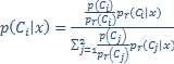	Posteriors using resampled data		Posteriors re-calibrated to original data
	P(Fraud)	P(No Fraud)	P(Fraud)	P(No Fraud)
Customer 1	0,100	0,900	0,004	0,996
Customer 2	0,300	0,700	0,017	0,983
Customer 3	0,500	0,500	0,039	0,961
Customer 4	0,600	0,400	0,057	0,943
Customer 5	0,850	0,150	0,186	0,814
Customer 6	0,900	0,100	0,267	0,733